Week of 11/5
(New page: Image:Squarewave.png Image:Sqwavexmgr.png) |
|||
| (21 intermediate revisions by one user not shown) | |||
| Line 1: | Line 1: | ||
| + | Here is the display of my oscilloscope when the input is a 1000 pulse per second output of a time-code generator. (The time-code generator is a device that locks to the 10 MHz output of an atomic clock and produces 1 Hz or 1 KHz pulse trains as well as human readable time synchronized to the atomic standard.) | ||
| + | |||
[[Image:Squarewave.png]] | [[Image:Squarewave.png]] | ||
| + | |||
| + | |||
| + | |||
| + | |||
| + | |||
| + | I imported the data and plotted it along with its periodogram. | ||
| + | |||
[[Image:Sqwavexmgr.png]] | [[Image:Sqwavexmgr.png]] | ||
| + | |||
| + | |||
| + | |||
| + | Notice that only the odd harmonics are present. | ||
| + | |||
| + | Here is a mathematica notebook that simulates this. | ||
| + | |||
| + | {{mathematica|filename=fouriertransformexamples.nb|title=lots of fourier transform examples}} | ||
| + | |||
| + | |||
| + | ---- | ||
| + | |||
| + | |||
| + | Sampling theorem. See 10/31/07 lecture notes | ||
| + | |||
| + | |||
| + | |||
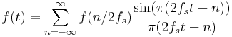
| + | We end up with | ||
| + | <math> | ||
| + | f(t) = \sum _ {n = - \infty} ^ \infty f(n/2f_s) \frac{\sin(\pi (2 f_s t -n))}{\pi (2 f_s t -n)} | ||
| + | |||
| + | </math> | ||
| + | |||
| + | |||
| + | This amounts to taking samples of the data every <math>1/2f_s</math> and multiplying them by a sinc function and adding up the results. | ||
| + | |||
| + | {{mathematica|filename=Sincinterpolation.nb|title=Sinc function interpolation via the samping theorem}} | ||
| + | |||
| + | |||
| + | |||
| + | |||
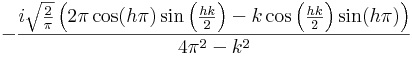
| + | Mathematica can find the fourier transform of a box function of width h centered on zero times <math>sin(2 \pi x)</math>: | ||
| + | |||
| + | <math>-\frac{i \sqrt{\frac{2}{\pi }} \left(2 \pi \cos (h \pi ) \sin \left(\frac{h k}{2}\right)-k \cos \left(\frac{h k}{2}\right) \sin (h \pi )\right)}{4 \pi ^2-k^2} | ||
| + | </math> | ||
| + | |||
| + | |||
| + | {{mathematica|filename=Sinpiece.nb|title=FT of finite sines}} | ||
| + | |||
| + | |||
| + | {{PDF|filename=11-7-07.pdf|title=11-7-07 notes}} | ||
| + | |||
| + | {{mathematica|filename=Timingfft.nb|title=timing the fft}} | ||
| + | |||
| + | |||
| + | {{mathematica|filename=Nyquist.nb|title=Nyquist exercise}} | ||
| + | |||
| + | |||
| + | |||
| + | {{mathematica|filename=Sounds.nb|title=cool sound examples with Mathematica}} | ||
| + | |||
| + | |||
| + | {{PDF|filename=11_9_07.pdf|title=11-9-07 notes}} | ||
| + | |||
| + | [[Image:3pointnyquist.png]] | ||
Latest revision as of 21:01, 6 December 2007
Here is the display of my oscilloscope when the input is a 1000 pulse per second output of a time-code generator. (The time-code generator is a device that locks to the 10 MHz output of an atomic clock and produces 1 Hz or 1 KHz pulse trains as well as human readable time synchronized to the atomic standard.)

I imported the data and plotted it along with its periodogram.

Notice that only the odd harmonics are present.
Here is a mathematica notebook that simulates this.
| |
Sampling theorem. See 10/31/07 lecture notes
We end up with
This amounts to taking samples of the data every 1 / 2fs and multiplying them by a sinc function and adding up the results.
| |
Mathematica can find the fourier transform of a box function of width h centered on zero times sin(2πx):
| |
| |
| |
| |
| |
| |
