PHGN-471 Fall-2011

Main Page

>

Physics Course Wikis

Modeling transport in thermoelectric materials via the Boltzmann transport equation

Advisor: Eric Toberer

Graduate Advisor: Aaron Martinez

Students: Kyle Conrad and Michael Dixon

Objective

Thermoelectric materials generate electricity from waste heat. Understanding electronic transport in semiconductors materials is critical for the development of a new generation of thermoelectric devices. These materials could potentially play a role in the world's future energy infrastructure. To date, modeling thermoelectric materials typically involves applying solutions to the Boltzmann transport equation within the limit of a single parabolic band. This senior design project will consider the effect of non parabolic bands, multiple bands, and inter-band scattering on the predicted properties of thermoelectric materials. The goal of this project is to use advanced transport expressions to determine an optimal thermoelectric band structure and develop guidelines for the selection of thermoelectric materials.

Statistical Mechanics

Distribution Functions

Distribution functions are functions that have little importance on their own, but when integrated form a meaningful value, like a probability. Four distribution functions will be examined; the Maxwell distribution, the Boltzmann distribution, the Fermi-Dirac distribution, and the Bose-Einstein distribution.

Boltzmann Distribution

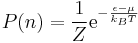
Consider a system of noninteracting particles. The Boltzmann distribution gives the probability of finding this system in a particular energy state, E, at temperature, T.

Suppose this system has two possible localized energy states E₁ and E₂. The probability these two states occurring at the same time is given by:

P_1,2 = P₁ * P₂

and the total energy of the system is given by:

E_1,2 = E₁ + E₂

From this it can be concluded that the probability of the system being in a particular energy state must be an exponential function.

$P_{1,2}=C*e^{-\beta(E_{1}+E_{2})}$

where,

$\beta=\frac{1}{k_{B}T}$

k_B is the Boltzmann constant and has been determined experimentally to be 1.381 * 10 ^{− 23}J / K. The Boltzmann distribution can now be written as:

$P_{r}=C*e^{-\frac{E_{r}}{k_{B}T}}$

P_r gives the probability of finding the system in state r with energy E_r at temperature T. Normalizing such that

∑	Pr = 1
r

gives:

$P_{r}=\frac{1}{Z}*e^{-\frac{E_{r}}{k_{B}T}}$

where Z is called the partition function.

Partition Function

Quote from Lindsay:

Once a partition function is calculated, all other equilibrium thermodynamic properties follow from minimizing the free energy of the system expressed in terms of the partition function

The grand partition function is given by:

$Z(T,V,\mu)=\sum_{Nr}^{}e^{\beta(\mu N-E_{Nr})}$

where μ is the chemical potential and Nr is the number of particles in a particular state.

Maxwell Distribution

Begin by considering an ideal gas. We will want to consider the motions of an individual molecule within the gas. More specifically, we will ask the question "What is the probability of a particular molecule moving at a given speed?". There are infinitely many speeds that the molecule may travel at, so the probability of the speed being a particular one is nearly zero. But relative to each other, some speeds are more probable than others so the relative probability of each speed must be considered. A plot of the relative probability for each speed v is shown below. This graph is normalized (the area underneath the curve is 1) so the area between two speeds is the probability that a molecule's speed is within the specified range.

INSERT GRAPH OF D(V)

The graph shows D(v), but what is D(v)? The equation below describes the two factors in the equation

$D(\textit{v})\propto(\text{Probability of molecule having }\vec{v})\times(\text{the number of vectors }\vec{v}\text{ corresponding to }\textit{v})$

The probability of a molecule having $\vec{v}$ is given by the Boltzmann Factor, $e^{\frac{-E(s)}{k_BT}}$. In the ideal gas, the total energy is due purely to the kinetic so $E(s)=\frac{1}{2}m\textit{v}^2$ The second factor in the equation can be found by considering 3 dimensional velocity space. In this space, the number of vectors $\vec{v}$ corresponding to v is the surface of a sphere of radius v.

Surface Area = 4πv²

D(v) is normalized, so the surface area, the Boltzmann factor, and a normalizing constant must be integrated from 0 to infinity and set equal to 1. Solving this for the normalizing constant completes Maxwell's distribution.

$D(v)=(\frac{m}{2 \pi k_B T})^{\frac{3}{2}} 4 \pi m v^2 e^{\frac{-mv^2}{2k_BT}}$

Fermi-Dirac and Bose-Einstein Distributions

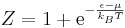
Consider a system of indistinguishable particles with only one particle state. The energy of the particle is defined as follows: ε when occupied, 0 when empty, and nε when occupied by n particles. The probability of a state being occupied by n particles is given by

$P(n) =\frac{1}{Z}\text{e}^{-\frac{\epsilon - \mu}{k_B T}}$

where Z is the grand partition function, μ is the chemical potential, and T is the temperature. Occupancy is the average number of particles in a state, and for this system is

$\bar{n}=\sum n P(n)$

Because fermions can not have the same set of quantum numbers as each other (Pauli Exclusion Principle) n can only be 1 or 0. As well the partition function for fermions is

$Z = 1 + \text{e}^{-\frac{\epsilon-\mu}{k_B T}}$

This generates the Fermi-Dirac distribution

$\bar{n}_{FD} = \frac{1}{e^{-\frac{\epsilon-\mu}{k_B T}}+1}$

For Bosons there is no restriction on available states, so n is any non-negative integer. The partition function for bosons is

$Z = \frac{1}{1-\text{e}^{\frac{\epsilon - \mu}{k_B T}}}$

Solving for the occupancy gives the Bose-Einstein distribution

$\bar{n}_{BE} = \frac{1}{e^{-\frac{\epsilon-\mu}{k_B T}}-1}$

Density of States

Now the system of N free electrons in occupied orbitals can be represented by points in a sphere in k-space. At absolute zero, the wave vector representing the radius of the sphere corresponds to the fermi energy. Each point corresponds to a distinct set of quantum numbers for a volume element (2π / L)³ in k-space. The total number of occupied orbitals in k-space.

$\frac{V}{3\pi^{2}}k_{F}^{3}=N$

or,

$k_{F}=\left(\frac{3\pi^{2}N}{V}\right)^{1/3}$

Putting equation 1.18 into equation 1.16 gives,

$E_{F}=\frac{\hbar^{2}}{2m}\left(\frac{3\pi^{2}N}{V}\right)^{2/3}$

Solving this equation for N and differentiating with respect to E gives an expression for the number of orbitals per unit energy. This quantity is called the density of states.

$g_{\epsilon}=\frac{V}{2\pi^{2}}\left(\frac{2m}{\hbar^{2}}\right)^{3/2}E^{1/2}$

This expression can be thought of as the quotient of the number of conduction electrons and the fermi energy.

The density of electrons at zero temperature is given by:

$n=\int dE g_{\epsilon}=\dfrac{k_{F}^{3}}{3\pi^{2}}$

The limits on your integral are from zero to the fermi energy. We con do the same thing for nonzero temperatures by multiplying by the fermi-dirac distribution. From this the low-temperature heat capacity of a fermi gas can be determined. (Kittel pg 100)

Independent, Free Electron Gas

1. Conduction electron move freely through the volume of the metal. Valence electrons and nuclei are fixed in place
2. Correctly predicts Ohm's law and electrical-thermal conductivity relation
3. Cannot explain heat capacity or magnetic susceptibilities of conduction electrons

Two important notes:

• Ion cores do not scatter conduction electrons is the cores form periodic potential. This is because matter waves propagate freely in a periodic structure. (See chapter 7 of Kittel)
• Electron-electron scattering is infrequent. (Consequence of Pauli exclusion)

Failures of this model:

1. Predicts a significant heat capacity from electrons
2. Does not account for variation of resistivity with temperature
3. Cannot explain why electron mean free path is so great

Energy Bands

Energy gaps cannot be derived from the free electron model. It can only be accomplished via the examination of the electron wave functions. K-values that satisfy the Bragg reflection condition create standing waves. These standing waves result in an aggregation of charge on the ion core and in between the cores. These two locations have a different value of potential energy and result in a gap of forbidden energies that is equal to twice the fourier component of the potential.

Fermi Energy

Consider a Fermi gas of N electrons at absolute zero. When considering spin $\left(m=\pm \frac{1}{2}\right)$, two electrons can be in any one orbital. The energy level of the most energetic electron of this system is termed the Fermi energy ε_f. It is only electrons located near the fermi energy that contribute to transport. This is because electrons move from state to state in steps of no more than k_BT.

Drude Model

Drude's model is constructed by applying the kinetic theory of gases to metals. In the kinetic theory of ideal gases molecules are assumed to be identical solid spheres which move in straight lines until a collision occurs. When a collision occurs, it is assumed that the collision takes no time. A few changes are made to move from the kinetic theory of ideal gases to the Drude model. In this model positive charges are fixed in place with valence electrons moving freely about, and are called conduction electrons. The inner core of electrons remain bonded to the nucleus and are considered a part of the fixed metal ion.

Collisions require major assumptions in Drude's model. Collisions are only between the ions and the electron, and the interactions besides collisions are neglected. The probability of a collision occurring in an infinitesimal amount of time is given by $\frac{1}{\tau}$, where τ is the relaxation time. The relaxation time is the average time that an electron will travel without experiencing a collision. During each collision, the electrons are assumed to reach thermal equilibrium with the ion which the collision occurred with. After the collision the electron is emitted with a random direction and a speed which is dependent on the temperature where the collision occurred. As basic as this model is, it does allow for calculation of the electrical and thermal conductivity as well as the hall coefficient.

Boltzmann Transport

Fermi Integrals

Defining the following integral will make expressions easier to understand.

$K_{l,m}=\int_{0}^{\infty} \epsilon^{l} \tau_{\epsilon}^{m}\vec{v_{g}}*\vec{v_{g}}g(\epsilon)\frac{\partial f_{0}}{\partial \epsilon}d\epsilon$

where σ is the electrical conductivity, α is the Seebeck coefficient, and κ is thermal conductivity. A rigorous discussion of the transport coefficients is necessary.

Electrical Current

The electrical current density is given by

$\vec{j}=-ne\vec{v}$

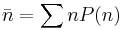
The number density is given by

$n = \int_0^\infty g(\epsilon)f(\epsilon) d\epsilon$

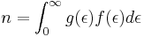
The current density may now be rewritten by plugging in the above equation for number density. When doing so, it must be remembered that the velocity is also a function of energy, and so it must be written inside of the integral.

$\vec{j} = - e \int_0^{\infty} \vec{v}_g g(\epsilon) f(\epsilon) d\epsilon$

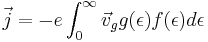
When considering a system at equilibrium, the current density is zero and the distribution function is the localized equilibrium distribution function, f⁰. Since the equilibrium current density equals zero, it may be subtracted from the current density with no consequence, because it is equal to zero. The result is

$\vec{j} = - e \int_0^{\infty} \vec{v}_g g(\epsilon) (f(\epsilon)-f^0(\epsilon)) d\epsilon$

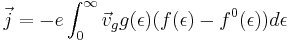
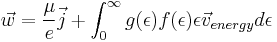
Using the Boltzmann transport equation to solve for (f(ε) − f⁰(ε)), the current density can be rewritten as

$\vec{j}=e\int_{0}^{\infty} \tau_{\epsilon}\vec{v}_{g} \vec{v}_{g}g(\epsilon)\left(\nabla\mu+\nabla T\frac{\epsilon-\mu}{T}\right)\frac{\partial f^{0}}{\partial \epsilon}d\epsilon$

Thermal Current

The thermal current is given by

$\vec{w} = \vec{w}_{energy}-\vec{w}_{convection}$

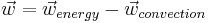
The energy current is caused by the flow of heat carrying electrons along a temperature gradient.

$\vec{w}_{energy} = u \vec{v}_{energy}$

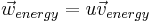
The energy density is given by

$\int^{\infty}_0 g(\epsilon) f(\epsilon) \epsilon \vec{v}_{energy} d\epsilon$

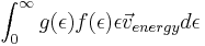
The convection current is the current caused by an external electric field.

$\vec{w}_{convection} = \mu \vec{v}_{conv.} n =\frac{-\mu}{e}\vec{j}$

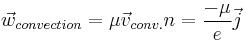
Using the above equations to solve for thermal current yields

$\vec{w} = \frac{\mu}{e} \vec{j} + \int^{\infty}_0 g(\epsilon) f(\epsilon) \epsilon \vec{v}_{energy} d\epsilon$

Similar to the process used in the derivation of the electrical current, we consider the steady state system. At steady state $\vec{w} \text{and} \vec{j}$ are 0, so the convection current on its own must equal zero. At equilibrium the distribution function is written as the equilibrium distribution function f⁰. Since this term equals zero, it may be subtracted from the thermal current with no consequence.

$\vec{w} = \frac{\mu}{e} \vec{j} + \int_0^{\infty} \vec{v}_{energy} \epsilon g(\epsilon) (f(\epsilon)-f^0(\epsilon)) d\epsilon$

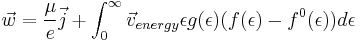
When substituting the Boltzman transport equation solved for f(ε) − f⁰(ε) the thermal current is written as

$\vec{w}=\frac{\mu}{e} \vec{j} + \int_{0}^{\infty} \tau_{\epsilon}\epsilon\vec{v}_{energy} \vec{v}_{g}g(\epsilon)\left(\vec{\nabla}\mu+\vec{\nabla} T\frac{\epsilon-\mu}{T}\right)\frac{\partial f^{0}}{\partial \epsilon}d\epsilon$

Transport Coefficients

Electrical Conductivity

Electrical conductivity is a quantity that relates a materials current response to an electric field. The constitutive relation describing this phenomena is known as ohm's law.

$\textbf{J}=\sigma \textbf{E}$

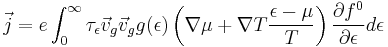
Taking $\textbf{E}=\frac{\nabla \mu}{e}$ and letting $\nabla T=0$ the current expression above we can write the conductivity as

$\sigma=e^{2}\int_{0}^{\infty} \tau_{\epsilon}\vec{v}_{g}*\vec{v}_{g}g(\epsilon)\frac{\partial f_{0}}{\partial \epsilon}d\epsilon$

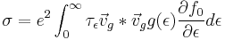
or

σ = e²K_0,1

Thermal Conductivity

Thermal conductivity describes a materials ability to conduct heat. There are multiple contributions to thermal conductivity.

K_T = κ_e + κ_ph + κ_bi + κ_pt

Phonon contribution

Electrical contribution

Photon contribution

Bipolar contribution

In the context of thermoelectrics, the goal is to reduce thermal conductivity.

Seebeck

The seebeck effect describes the creation of a voltage across a material in response to a temperature gradient. From mahan book chapter 11. Consider a bar of material of length L. Assume a temperature gradient such that

$\nabla T=\frac{\Delta T}{L}$

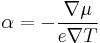
The material is insulated so, $\textbf{J}=0$. Then there will be electric field between the ends given by

$\textbf{E}=-\frac{\Delta V}{L}$

The ratio of these quantities is a property intrinsic to a material and described via the Seebeck coefficient.

$\alpha=\frac{\Delta V}{\Delta T}$

Letting $\textbf{E}=\frac{\nabla\mu}{e}$This can also be written as:

$\alpha=-\frac{\nabla\mu}{e \nabla T}$

From this definition for the Seebeck coefficient, we are now in a position to derive an expression for this quantity via more rigorous expressions for current. Consider the expression for electrical current shown in a previous section. Letting $\textbf{J}=0$

$0=e\int_{0}^{\infty} \tau_{\epsilon}\vec{v}_{g}*\vec{v}_{g}g(\epsilon)\left(\nabla\mu+\nabla T\frac{\epsilon-\mu}{T}\right)\frac{\partial f_{0}}{\partial \epsilon}d\epsilon$

Now distribute through the quantity in parentheses

$0=e\int_{0}^{\infty} \tau_{\epsilon}\vec{v}_{g}*\vec{v}_{g}g(\epsilon)\nabla T\frac{\epsilon-\mu}{T}\frac{\partial f_{0}}{\partial \epsilon}d\epsilon-e\int_{0}^{\infty} \tau_{\epsilon}\vec{v}_{g}*\vec{v}_{g}g(\epsilon)\nabla\mu\frac{\partial f_{0}}{\partial \epsilon}d\epsilon$

This expression in terms of the K integrals previously defined is

$0 = \Delta\mu K_{0,1} + \frac{\nabla T}{T} K_{1,1} + \mu\frac{\nabla T}{T}K_{0,1}$

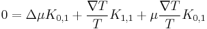
Now solve for $\frac{\nabla \mu}{\nabla T}$ and the Seebeck coefficient can be written as

$\alpha=\frac{1}{eT}\left[\mu-\frac{K_{1,1}}{K_{0,1}}\right]$

Physically the Seebeck effect can be explained by the propagation of electrons from the hot side of the material to the cold side.

Peltier

This process is analogous to the seebeck effect. Some materials will absorb heat when a current is passed through it. The peltier coefficient can be defined as the ratio of the heat carried by the charges to the current across the material.

$\Pi=\frac{Q}{I}$

The peltier coefficient can also be related to the seebeck coefficient:

Π = αT

Hall

Examination of the Hall effect provides valuable information regarding the conduction properties of semiconductors.

Quote from Lindberg paper: "The Hall effect provides a direct measurement of the carrier type and concentration and, in conjunction with the resistivity, yields the mobility."

In addition, the Hall effect can give an accurate measurement of the impurity level. Consider a substance carrying a current in the x-direction with a magnetic field applied in the z-direction. An E-field will occur in the y-direction and is called the Hall field. The Hall field will be proportional to the product of the current density and the magnitude of the applied magnetic field. The constant of proportionality is the Hall Coefficient.

E_H = − RJH

The Hall effect allows for the determination of carrier concentration and mobility. The Hall effect can be explained from a semi-classical standpoint.

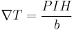
Nernst

Consider a sample with a thermal current in the x-direction and a magnetic field in the z-direction. An electric field will be induced in the y-direction.

$E_{N}=Q\frac{wH}{K}$

Where Q is the Nernst coefficient, w is the thermal current, H is the magnetic field perpendicular to current flow, and K is the thermal conductivity of the sample.

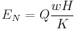
Ettingshausen

Consider a sample with a current flow in the x-direction and an applied electric field in the z-direction. If this occurs a temperature gradient will appear in y-direction.

$\nabla T=\frac{PIH}{b}$

Where P is the Ettingshausen coefficient, I is the current, H is the magnetic field perpendicular to current flow, and b is the thickness of the sample.

Righi-Leduc

This effect produces a temperature gradient in the y-direction when a thermal current is applied in the x-direction, and a magnetic field is applied in the z-direction.

$\frac{\Delta T}{a}=\frac{S \omega H}{K}$

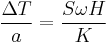
Where a is the width of the sample, ω is the thermal current and K is the thermal conductivity of the sample.

Thermoelectrics

Figure of Merit

It is now worth noting the thermoelectric figure of merit zT.

$zT=\frac{\sigma \alpha^{2}}{\kappa}T$

Maximizing this quantity can be difficult considering the somewhat contradictory requirements of high seebeck, high conductivity, and low thermal conductivity. Many efforts have focused on the reduction of the lattice component of thermal conductivity.

This figure of merit has led researchers to pursue materials that have high electrical conductivities such as those associated with rigid crystals, and low thermal conductivity such as amorphous materials. This has led to the term phonon glass, electron crystal.

References

Texts

1. Schroeder, Daniel V. Thermal Physics. 2000
2. Kittel, Charles. Solid State Physics. 2005
3. Griffiths. David. Introduction to Quantum Mechanics. 2005
4. Mahan, Gerald.Condensed Matter in a Nutshell. 2010
5. Lindsay, S.M. Introduction to Nanoscience. 2009
6. Nolas, G.S. Thermoelectrics: Basic Principles and New Materials Developments. 1962
7. Ashcroft and Mermin. Solid State Physics. 1976

Papers

1. Snyder J.G. & Toberer E.S., Complex Thermoelectric Materials. Nature, 7 105-114 (2008).
2. Mahan G.D., The Best Thermoelectric. 93 7436-7439 (1996).
3. Zevalkink A & Toberer E.S., Ca₃AlSb₃: An inexpensive, non-toxic thermoelectric material for waste heat recovery. Energy Environ. Sci., 4, 510-518 (2011).
4. Lindberg O, Hall Effect. (1952).