Modern 2:Measurements and Eigenstates
(→Observables) |
|||
| (24 intermediate revisions by 3 users not shown) | |||
| Line 1: | Line 1: | ||
| + | {{Start Hierarchy|link=Course Wikis|title=Course Wikis}} | ||
| + | {{Hierarchy Item|link=Physics Course Wikis|title=Physics Course Wikis}} | ||
| + | {{Hierarchy Item|link=Modern 2|title=Modern 2}} | ||
| + | {{End Hierarchy}} | ||
| + | |||
===states with precisely known energy=== | ===states with precisely known energy=== | ||
Here is the Schrodinger equation for a nonrelativistic particle in an external, time-independent potential | Here is the Schrodinger equation for a nonrelativistic particle in an external, time-independent potential | ||
| Line 10: | Line 15: | ||
I'm going to rewrite this using a hat over the momentum to indicate the fact that it is really an operator: | I'm going to rewrite this using a hat over the momentum to indicate the fact that it is really an operator: | ||
| − | <math> \frac{\hbar}{i} \nabla = \hat{\ | + | <math> \frac{\hbar}{i} \nabla = \hat{\mathbf{p}} </math> |
Let us define an operator for the total energy (kinetic plus potential). This is called the Hamiltonian | Let us define an operator for the total energy (kinetic plus potential). This is called the Hamiltonian | ||
| Line 16: | Line 21: | ||
<math> \hat{H} = \frac{{\vec{p}}^2}{2m} + \hat{V} </math> | <math> \hat{H} = \frac{{\vec{p}}^2}{2m} + \hat{V} </math> | ||
| − | <math> = - \frac{\hbar^2}{2 m} \nabla^2 | + | <math> = - \frac{\hbar^2}{2 m} \nabla^2 + V(\vec{r}) </math> |
Using this we can rewrite the Schrodinger equation as | Using this we can rewrite the Schrodinger equation as | ||
| Line 22: | Line 27: | ||
'''(3.16)''' <math> i \hbar \frac{\partial}{\partial t} \psi(\vec{r}, t) = \hat{H} \psi(\vec{r}, t) </math> | '''(3.16)''' <math> i \hbar \frac{\partial}{\partial t} \psi(\vec{r}, t) = \hat{H} \psi(\vec{r}, t) </math> | ||
| − | Normally we expect that the result repeated measurments of systems prepared identically will yield a spread of results. But there are clearly some measurement which lead to very precise and repeatable measurements, such as spectral lines, narrow-band laser frequencies, etc. So let us consider the case in which the time dependence of the wave function is a constant frequency sinusoid. I.e., suppose that | + | Normally we expect that the result of repeated measurments of systems prepared identically will yield a spread of results. But there are clearly some measurement which lead to very precise and repeatable measurements, such as spectral lines, narrow-band laser frequencies, etc. So let us consider the case in which the time dependence of the wave function is a constant frequency sinusoid. I.e., suppose that |
<math> | <math> | ||
| Line 36: | Line 41: | ||
This is an example of an eigenvalue/eigenfunction problem. <math>E ,\ </math> is an eigenvalue of the operator <math> \hat{H} ,\ </math> associated with the eigenvector <math> \psi(\vec{r}) ,\ </math>. | This is an example of an eigenvalue/eigenfunction problem. <math>E ,\ </math> is an eigenvalue of the operator <math> \hat{H} ,\ </math> associated with the eigenvector <math> \psi(\vec{r}) ,\ </math>. | ||
| − | |||
| − | |||
===examples of precisely determined measurements=== | ===examples of precisely determined measurements=== | ||
[http://en.wikipedia.org/wiki/Spectral_line spectral lines] | [http://en.wikipedia.org/wiki/Spectral_line spectral lines] | ||
| + | |||
| + | [http://www.phys.ufl.edu/courses/phy4803L/balmer/balmer.html optical spectroscopy] | ||
| + | |||
| + | [http://www.astro.ucla.edu/~wright/fluxplot.html flux plot] with nice java applet | ||
| + | |||
| + | [http://www.cem.msu.edu/~reusch/VirtualText/Spectrpy/nmr/nmr1.htm nice NMR page] | ||
===Observables=== | ===Observables=== | ||
| Line 50: | Line 59: | ||
'''(3.5)''' <math> \langle a \rangle _ t = \int \psi^*(\vec{r},t) \left[ \hat{A} \psi(\vec{r},t) \right] d^3 r </math> | '''(3.5)''' <math> \langle a \rangle _ t = \int \psi^*(\vec{r},t) \left[ \hat{A} \psi(\vec{r},t) \right] d^3 r </math> | ||
| − | To understand this equation suppose that <math> \psi ,\ </math> were an ordinary real vector | + | To understand this equation suppose that <math> \psi ,\ </math> were an ordinary real vector and <math>A \ </math> a matrix. Then we would write the RHS as |
<math> \left( \psi, A \psi \right) \ </math> | <math> \left( \psi, A \psi \right) \ </math> | ||
| Line 59: | Line 68: | ||
Proof: <math> \left(A \psi, \psi \right) = | Proof: <math> \left(A \psi, \psi \right) = | ||
| − | \sum _ i ( \sum _ j A_{ij} \psi_j ) \psi_i = \sum _ j \psi_j (\sum_i A_{ij} \psi_i) | + | \sum _ i ( \sum _ j A_{ij} \psi_j ) \psi_i = \sum _ j \psi_j (\sum_i A_{ij} \psi_i) |
| + | |||
= \sum _ j \psi_j (\sum_i A^T_{ji} \psi_i) = \left( \psi, A^T \psi \right) = | = \sum _ j \psi_j (\sum_i A^T_{ji} \psi_i) = \left( \psi, A^T \psi \right) = | ||
\left( \psi, A \psi \right) \ </math> | \left( \psi, A \psi \right) \ </math> | ||
| Line 65: | Line 75: | ||
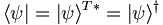
But this is for real vectors. For complex vectors, as we discussed in the last class, we need a complex conjugate in the inner product in order that the inner product of a vector with itself be real. All of these considerations led Dirac to invent a new notation for function inner products such as '''(3.5)'''. In Dirac's '''bra-ket''' notation '''(3.5)''' becomes: | But this is for real vectors. For complex vectors, as we discussed in the last class, we need a complex conjugate in the inner product in order that the inner product of a vector with itself be real. All of these considerations led Dirac to invent a new notation for function inner products such as '''(3.5)'''. In Dirac's '''bra-ket''' notation '''(3.5)''' becomes: | ||
| − | <math> \langle \psi | A \psi \rangle \ </math> | + | <math> \langle \psi | \hat{A} | \psi \rangle \ </math> |
which for self-adjoint operators is equivalent to | which for self-adjoint operators is equivalent to | ||
| − | <math> \langle A \psi |\psi \rangle \ </math> | + | <math> \langle \hat{A} \psi |\psi \rangle \ </math> |
| − | In this notation, the ket vector <math> |\psi\rangle | + | In this notation, the ket vector <math> |\psi\rangle </math> is different than the bra vector |
<math> \langle \psi |</math>. In fact, we have | <math> \langle \psi |</math>. In fact, we have | ||
| − | <math> \langle \psi | = | + | <math> \langle \psi | = |\psi\rangle ^{T*} = |\psi\rangle ^ \dagger </math> |
| + | |||
| + | Suppose <math> \alpha \ </math> and <math> \beta \ </math> represent two states of the system. Then the inner product of these two states is <math> \langle \alpha | \beta \rangle = \langle \beta | \alpha \rangle^* \ </math>. In coordinate | ||
| + | space representation we would write this inner product as an integral (in one-dimension) as | ||
| + | |||
| + | <math> \int \psi ^* _\alpha (x) \psi_\beta (x) dx </math>. | ||
| + | |||
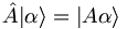
| + | Here is a minor, slightly picky bit of notation. We know that operators map vectors into vectors. Hence they map, say, ket-vectors into ket-vectors. So we denote by <math> |A \alpha\rangle</math> the ket which is obtained by operating on | ||
| + | <math> |\alpha\rangle</math> by the operator <math> \hat A </math>: | ||
| + | |||
| + | <math> \hat{A} | \alpha \rangle = | A \alpha \rangle </math> | ||
| + | |||
| + | |||
| + | ===operators have different algebraic properties than numbers or functions=== | ||
| + | |||
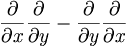
| + | Consider an operator equation | ||
| + | |||
| + | <math> \frac{\partial}{\partial x} \frac{\partial}{\partial y} - \frac{\partial}{\partial y} \frac{\partial}{\partial x} </math> | ||
| + | |||
| + | if these were numbers then this would clearly be zero. But for operators, this is shorthand for | ||
| + | |||
| + | <math> \left[ \frac{\partial}{\partial x} \frac{\partial}{\partial y} - \frac{\partial}{\partial y} \frac{\partial}{\partial x} \right] f(x,y) </math> | ||
| + | |||
| + | where f is some well-behaved function. In Quantum Mechanics a combination such as <math> AB - BA \ </math> | ||
| + | is called a commutator. We know from ordinary calculus that the commutator of partial derivatives is zero. | ||
| + | |||
| + | <math> [\frac{ \partial}{\partial x} , \frac{\partial}{\partial y}] = 0</math> | ||
| + | |||
| + | But what about | ||
| + | |||
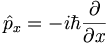
| + | <math> [\frac{ \partial}{\partial x}, x] </math> ? | ||
| + | |||
| + | HW not to be turned in: show that | ||
| + | |||
| + | <math> [\hat{x}, \hat{p}_x] = i \hbar \hat{I} </math> | ||
| + | |||
| + | where | ||
| + | |||
| + | <math> \hat{p}_x = -i \hbar \frac{\partial}{\partial x} </math> | ||
| + | |||
| + | |||
| + | |||
| + | |||
| + | ===orthogonality of the eigenfunctions of self-adjoint operators=== | ||
| + | |||
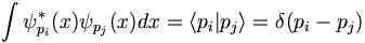
| + | '''HW not to be turned in''': prove the following. If <math> \psi _1 </math> and <math> \psi _2 </math> are two eigenfunctions of a self-adjoint operator with '''different''' eigenvalues, then <math> \psi _1 </math> and <math> \psi _2 </math> are orthogonal. I.e., <math> \langle \psi_1 | \psi_2 \rangle = 0 </math>. An important example of this is the following: | ||
| + | |||
| + | Take | ||
| + | <math>\psi_{p_j} = \frac{1}{\sqrt{2 \pi \hbar}} e^{ip_j x/\hbar}</math> to be the normalized momentum eigenfunction for a free particle with momentum <math>p_j</math> then | ||
| + | |||
| + | <math> \int \psi ^* _{p_i}(x) \psi _{p_j}(x) dx = \langle p_i | p_j \rangle = \delta(p_i - p_j) </math> | ||
| + | |||
| + | |||
| + | |||
| Line 101: | Line 164: | ||
which then gives (using Einstein's relation) | which then gives (using Einstein's relation) | ||
| − | <math> \Delta E \Delta t \geq h | + | <math> \Delta E \Delta t \geq h </math> |
| − | + | ||
| − | + | ||
Latest revision as of 07:15, 25 January 2007
| Course Wikis | > | Physics Course Wikis | > | Modern 2 |
Contents |
states with precisely known energy
Here is the Schrodinger equation for a nonrelativistic particle in an external, time-independent potential
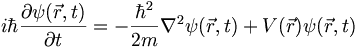
We'll be working on this equation for the rest of the semester! In the homework you will prove that the position-space represnetation of the momentum operator is given by
(3.9) 
I'm going to rewrite this using a hat over the momentum to indicate the fact that it is really an operator:

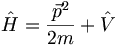
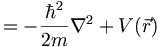
Let us define an operator for the total energy (kinetic plus potential). This is called the Hamiltonian
Using this we can rewrite the Schrodinger equation as
(3.16)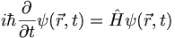
Normally we expect that the result of repeated measurments of systems prepared identically will yield a spread of results. But there are clearly some measurement which lead to very precise and repeatable measurements, such as spectral lines, narrow-band laser frequencies, etc. So let us consider the case in which the time dependence of the wave function is a constant frequency sinusoid. I.e., suppose that

A constant frequency means a constant energy. So if we plug this kind of wavefunction into 3.16 the Schrodinger equation becomes
(3.17)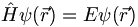
This is an example of an eigenvalue/eigenfunction problem.  is an eigenvalue of the operator
  associated with the eigenvector
  .
.
examples of precisely determined measurements
flux plot with nice java applet
Observables
Study Principle 3.1 in the book carefully. It says that for any physical quantity  (e.g., position, angular momentum, energy, etc) there is an operator
  which we call the observable associated with
, and that this operator is a linear Hermitian (self-adjoint) operator. We will denote by the lower case
which we call the observable associated with
, and that this operator is a linear Hermitian (self-adjoint) operator. We will denote by the lower case  the result of a measurement of . Then the expected value of such a measurement at any time
  is given by
(3.5)![\langle a \rangle _ t = \int \psi^*(\vec{r},t) \left[ \hat{A} \psi(\vec{r},t) \right] d^3 r](/csm/wiki/images/math/d/f/d/dfd4ba324b7e7bb779d5aea18baf7a4b.png)
To understand this equation suppose that  were an ordinary real vector and a matrix. Then we would write the RHS as

For a symmetric matrix this is equal to

Proof: 
But this is for real vectors. For complex vectors, as we discussed in the last class, we need a complex conjugate in the inner product in order that the inner product of a vector with itself be real. All of these considerations led Dirac to invent a new notation for function inner products such as (3.5). In Dirac's bra-ket notation (3.5) becomes:

which for self-adjoint operators is equivalent to

In this notation, the ket vector  is different than the bra vector
 . In fact, we have
Suppose  and
and  represent two states of the system. Then the inner product of these two states is
  . In coordinate
space representation we would write this inner product as an integral (in one-dimension) as
. In coordinate
space representation we would write this inner product as an integral (in one-dimension) as
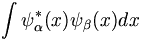 .
.
Here is a minor, slightly picky bit of notation. We know that operators map vectors into vectors. Hence they map, say, ket-vectors into ket-vectors. So we denote by  the ket which is obtained by operating on
 by the operator
  :
:
operators have different algebraic properties than numbers or functions
Consider an operator equation
if these were numbers then this would clearly be zero. But for operators, this is shorthand for
![\left[ \frac{\partial}{\partial x} \frac{\partial}{\partial y} - \frac{\partial}{\partial y} \frac{\partial}{\partial x} \right] f(x,y)](/csm/wiki/images/math/6/f/8/6f88f36649958abbea8d03f59b80d7dd.png)
where f is some well-behaved function. In Quantum Mechanics a combination such as  is called a commutator. We know from ordinary calculus that the commutator of partial derivatives is zero.
![[\frac{ \partial}{\partial x} , \frac{\partial}{\partial y}] = 0](/csm/wiki/images/math/4/2/d/42dd37fe9abc307e1b7bee30f001f5f8.png)
But what about
![[\frac{ \partial}{\partial x}, x]](/csm/wiki/images/math/7/d/5/7d51bbdb8e192e14f03ee42cc057f514.png) ?
?
HW not to be turned in: show that
![[\hat{x}, \hat{p}_x] = i \hbar \hat{I}](/csm/wiki/images/math/0/a/2/0a267fe0eaddf26fdd5006f12ef2e598.png)
where
orthogonality of the eigenfunctions of self-adjoint operators
HW not to be turned in: prove the following. If ψ1 and ψ2 are two eigenfunctions of a self-adjoint operator with different eigenvalues, then ψ1 and ψ2 are orthogonal. I.e., 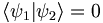 . An important example of this is the following:
Take
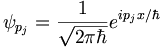 to be the normalized momentum eigenfunction for a free particle with momentum pj then
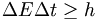
digression on the time/energy uncertainty relation
We have seen that in general if N copies of a system are prepared in identical states, then the result of any measurement will have a statistical spread of values. Further, there is a fundamental connection between the uncertainty of an observable and that of its Fourier transform pair. E.g.,
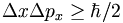
It would be nice if we could expect something like
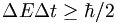
to be true, but it's not obvious.
John Baez on the time/energy uncertainty relation
One of the reasons it's not obvious is that there while there is an energy operator in QM (the Hamiltonian), there is no time operator in QM!
It turns out that from the Fourier transform ideas we've talked about you can show that:
which then gives (using Einstein's relation)