Bnibling/Acoustic Lab

(Difference between revisions)

Jump to: navigation, search

Revision as of 05:34, 4 December 2007

Harmonics

Barrett Nibling

December 4th, 2007

Abstract

This experiment dealt with the unique frequency patterns, known as harmonics, that sound produces in a resonator. Using white noise generated by a computer and transmitted through a speaker into our resonant cavity, a pipe, and at the other end was placed a microphone to record the outgoing frequencies. Using the geometry of the pipe and derived equations, theoretical values were calculated were calculated and compared to the measured values. The experimental data was within <insert %>% of the theoretical data.

List of Figures

Introduction

Sound produces unique frequency patterns when travelling through a resonant cavity, such as a tube, known as harmonics. These patterns depend on the frequencies sent into the body, the material, but more importantly the geometry of the structure. A computer was used to produce sound waves in the form of white noise through a speaker into one end of the cavity and by placing a microphone recording the frequency patterns on the other end, we could record the data on the computer for analysis. The computer software represents the data as a plot and the patterns on a graph shows the resonant peaks which occured in the cavity. These peaks can then be compared to expected peaks by using previously derived equations for the tubes we used. The derived peaks and the expected peaks were then compared and were found to agree within experimental error.

Theory

Procedure

Schematic of Harmonics Apparatus

Results

Helium, d=1/600mm, m=1
Color	$θ d i f f$ (degrees)	$λ$ (nm)	Error (nm)	Published $λ$ (nm)
Purple	15.6	448.0	$\pm$ 2.0	447.148
Teal	16.4	470.3	$\pm$ 2.0	471.314
Green	17.2	492.6	$\pm$ 2.0	492.193
Green	17.5	500.9	$\pm$ 2.0	501.567
Yellow//Orange	20.7	588.8	$\pm$ 2.0	587.562
Red	23.6	666.9	$\pm$ 2.0	667.815
Dim Red	25.1	706.7	$\pm$ 1.9	???

Error Analysis

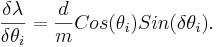
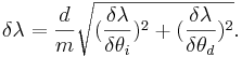
$\frac{\delta \lambda}{\delta \theta_{i}}=\frac{d}{m}Cos(\theta_{i}) Sin({\delta \theta_{i}}).$

Then the total error is the sum of the two partial derivatives added in quadrature,

$\delta \lambda=\frac{d}{m} \sqrt{(\frac{\delta \lambda}{\delta \theta_{i}})^{2}+(\frac{\delta \lambda}{\delta \theta_{d}})^{2}}.$

Conclusion

References

[1]

[2]

@@ Line 14: / Line 14: @@
 == Introduction ==
+Sound produces unique frequency patterns when travelling through a resonant cavity, such as a tube, known as harmonics. These patterns depend on the frequencies sent into the body, the material, but more importantly the geometry of the structure. A computer was used to produce sound waves in the form of white noise through a speaker into one end of the cavity and by placing a microphone recording the frequency patterns on the other end, we could record the data on the computer for analysis. The computer software represents the data as a plot and the patterns on a graph shows the resonant peaks which occured in the cavity. These peaks can then be compared to expected peaks by using previously derived equations for the tubes we used. The derived peaks and the expected peaks were then compared and were found to agree within experimental error.
 == Theory ==

Bnibling/Acoustic Lab

Revision as of 05:34, 4 December 2007

Contents

Abstract

List of Figures

Introduction

Theory

Procedure

Results

Error Analysis

Conclusion

References

Personal tools

Namespaces

Variants

Views

Actions

Search

Navigation

Toolbox