Bnibling/Acoustic Lab

Harmonics

Barrett Nibling

December 4th, 2007

---

Abstract

This experiment dealt with the unique frequency patterns, known as harmonics, that sound produces in a resonator. Using white noise generated by a computer and transmitted through a speaker into our resonant cavity, a pipe, and at the other end was placed a microphone to record the outgoing frequencies. Using the geometry of the pipe and derived equations, theoretical values were calculated were calculated and compared to the measured values. The experimental data was within 1% of the theoretical data.

List of Figures

[1] Schematic of Harmonics Apparatus

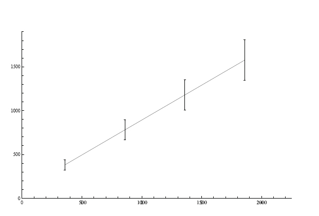
[2]Measured Frequencies Compared to Theoretical Frequencies Graph

Introduction

Sound produces unique frequency patterns when travelling through a resonant cavity, such as a tube, known as harmonics. These patterns depend on the frequencies sent into the body, the material, but more importantly the geometry of the structure. A computer was used to produce sound waves in the form of white noise through a speaker into one end of the cavity and by placing a microphone recording the frequency patterns on the other end, we could record the data on the computer for analysis. The computer software represents the data as a plot and the patterns on a graph shows the resonant peaks which occurred in the cavity. These peaks can then be compared to expected peaks by using previously derived equations for the tubes we used. The derived peaks and the expected peaks were then compared and were found to agree within experimental error.

Theory

When a sound wave of a specific frequency enters a cavity, such as a musical instrument, the cavity will absorb the energy of the wave and produce a standing wave pattern that matches the resonant frequency. This only occurs when the specific frequency of the waves entering the system are close to the frequency of the acoustic resonance of the cavity. These resonant frequencies are known as harmonics. Each system of this type will have an infinite number of harmonics. The lowest frequency harmonic is called the fundamental frequency. Each harmonic following is a nth multiple of the fundamental frequency, known as the nth harmonics.

The constraint that determines the harmonic frequencies is the system itself. In the case of a pipe, which was used for our experiment, the resonance depends mainly on the length of the pipe. Since the pipe is open at both ends, the following previously derived equation can be used to approximate the harmonic frequency,

$f = \frac{n v_s}{2 L},$

where n is a positive constant integer, v_s is the speed of sound, and L is the length of the pipe. The speed of sound is given to be at 334 m/s[1]. This isn't the best equation that matches the model. The radius of the pipe effectively makes the pipe long, the bigger the radius, the more air the waves must travel through[2]. To account for this, the end correction factor of 0.6R, R being the radius of the pipe, must be implemented into the equation (1). Giving the following new equation,

$f = \frac{n v_s}{2(L+0.6R)}.$

Calculations from this equation will than be compared with the data acquired from the microphone.

Procedure

1. Log on the computer and start up Baudline

2. Begin emitting white noise from the speaker

3. Place one opening of the pipe in front of the speaker and place the microphone on the opposite opening as shown in the figure below

Schematic of Harmonics Apparatus[3]

4. Save the data, making sure to substract the baseline from the white noise.

5. Analyze the data into a plot and observe the resonant peaks that occur.

Results

The following table and graph are the results acquired from a pipe of Length 38.3cm and Radius 13.4mm

Data Table for Pipe 1, L=38.3cm $\pm$ .05cm and R=13.4mm $\pm$ .05mm

n	Theoretical Frequency (Hz)	Theoretical Frequency with End Correction (Hz)	Error with End Correction (Hz)	Measured Frequency (Hz)
1	436.0	427.1	$\pm$ 6.4	421.9
2	872.1	854.1	$\pm$ 12.8	843.75
3	1308.1	1281.2	$\pm$ 19.2	1283.2
4	1744.1	1708.3	$\pm$ 25.7	1699.2

Measured Frequencies Compared to Theoretical Frequencies

The following table is the data collected from a smaller pipe of Length L = 18.2cm and Radius 24.55mm.

Data Table for Pipe 2, L=18.2cm $\pm$ .05cm and R=24.55mm $\pm$ .05mm

n	Theoretical Frequency (Hz)	Theoretical Frequency with End Correction (Hz)	Error with End Correction (Hz)	Measured Frequency (Hz)
1	917.6	848.9	$\pm$ 12.9	855.5
2	1835.2	1697.8	$\pm$ 25.8	1687.3
3	2752.8	2546.6	$\pm$ 38.7	2537.4
4	3670.3	3395.5	$\pm$ 51.6	3416.0

Error Analysis

For the error analysis, there were three variables associated with error, L, R, and v. The following are the three partial errors for each variable,

$\frac{\delta f}{\delta v_c}=\frac{n \delta v_s}{2(L+0.6R)},$

$\frac{\delta f}{\delta L}=-\frac{n v_s \delta L}{(L+0.6R)^2},$

and

$\frac{\delta f}{\delta R}=-\frac{0.3 n v_s \delta R}{(L+0.6R)^2}.$

Then the total error is the sum of the three partial derivatives added in quadrature,

$\delta f = \sqrt{(\frac{\delta f}{\delta v_c})^{2}+(\frac{\delta f}{\delta L})^{2}+(\frac{\delta f}{\delta R})^{2}}.$

The value for δL is 0.05cm, for δR is 0.05mm, and for δv_s was 5 m/s since speed of sound varies at different altitudes.

Conclusion

For the experiment, the measured data fit well with the theoretical values. All values calculated were within 1% error of the theoretical values. Also, it determined that there was an increase in accuracy with the end correction. Without the end correction, the data would have been off by almost an order of magnitude at some frequencies. Surprisingly the biggest source error came associated with the speed of sound. But it is minimal since there is plenty of background to determine the speed at different altitudes.

References

[1] Wikipedia, “Speed of Sound“, en.wikipedia.org/wiki/Speedofsound

[2] "FAQ in music acoustics: The End Correction", http://www.phys.unsw.edu.au/jw/musFAQ.html#end

[3] “Modes in a Resonator“, http://ticc.mines.edu/csm/wiki/images/5/5b/Acoustics_07.pdf