Basics of Linear Algebra: Things you are supposed to know before Modern II

There are a few basic things you are supposed to know about Linear Algebra by spring of junior year. Most of this is covered in Math Physics, but that class has a lot of territory to cover, much of it seemingly unrelated to the rest, and as such many people have only very basic knowledge coming out of that class, and much of that is forgotten all too easily. This is a simple guide which illustrates many of the concepts at a basic level to clear up any confusion that may occur going into Modern Physics. The official Wikipedia pages dealling with the subject are: Vector Space Matrices Transpose Adjoint Matrix Multiplication Basis Spectral Theorem

Matrices and Vectors

There are three kinds of object you need to deal with. The first two are scalars and vectors, and the third is matrices. As you already know, scalars are just numbers, vectors are lists of numbers (like matrices but one dimension is of length one), and matrices are grids of numbers. These are all "tensors". There are more, higher ranked tensors, like 3-D grids of numbers, but those aren't so useful just now. Here are three generic objects:

x = x₁

Note that matrices are usually denoted by capital letters, and that operators (which are matrices) have hats. Also, rows are the first index, while columns are the second. Finally, note that the word "vector" by default implies a column vector, one with one column. The transpose of a column vector is a row vector.

Transpose

The transpose of a matrix is simply the matrix with its rows turned into its columns, and vice versa. Another way to put it is that the matrix is reflected about its diagonal (the sequence of entries from top-left to bottom-right).

Also: 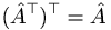$(\hat{A}^{\top})^{\top}=\hat{A}$

Adjoint

The adjoint of a matrix is simply the complex conjugate of the transpose. When one is using complex numbers almost all techniques that are typically used with the transpose of a matrix are instead used with the adjoint.

Matrix Multiplication

When two matrices are multiplied, each row (m) of the first is multiplied by each column (n) of the second, and the results are placed in the mth row and nth column of a new matrix. This multiplication is the vector dot product (the sum of the products of the nth row term with the nth column term). There are a few key points here. Firstly, since the columns of a matrix are generally not the same as its rows, matrix multiplication does not commute: $\hat{A} \hat{B}\neq \hat{B} \hat{A}$. However, it is true that 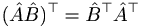$(\hat{A} \hat{B})^{\top}=\hat{B}^{\top} \hat{A}^{\top}$. A second point is that matrix multiplication only works like this if the number of columns in the first matrix equals the number of rows in the second. Thirdly, the product matrix has the same number of rows as the first matrix and the same number of columns as the second.

Finally, since vectors are just matrices with some number L rows and 1 column, all these rules apply to vectors. The dot product can therefore be described in terms of vector multiplication, as $\vec{v_{1}}^{\top} \vec{v_{2}}$. This dot product is a 1x1 matrix, which is just a scalar to us. There are three main points to be made here, from the standpoint of Modern II.

• Firstly, in bra-ket notation the adjoint takes the place of the transpose here (which is necessary when working with complex numbers).
• Secondly, column (normal) vectors are exactly the same thing as kets, and row (adjoint) vectors are bras. Bra-ket notation essentially exists because you don't always know the exact numbers in a vector (or the numbers might change, in fact), and bra-ket notation lets you say something about the properties of operators and vectors without knowing anything specific about their actual contents.
• Thirdly, $\vec{v_{1}} \vec{v_{2}}^{\top}$ is not the dot product, but actually a rather different object (sometimes called an "outer" product). Specifically, for vectors of length L, it is an LxL matrix. So although inner products are scalars and can move anywhere in an equation, vectors that are not moving as an inner product can not change order of multiplication. Neither can operators unless some symmetry condition lets them do so.

A Word on Basis

Basis refers to component vectors you can use to build up a space. For example, one can build a normal 3-D space out of the x, y, and z vectors. Although you may not need it quite yet it is important to know that in any given space there are many different basis sets that can be used (in the case of 3-D space, one could rotate one's axes to get a new set of basis vectors, for example).

Eigenvalues and Eigenvectors

In quantum mechanics our primary concern with operators is that they can be applied to a state vector and "spit out" another state vector. This is shown simply with the equation $\hat{A}\vec{x}=\vec{y}$. One very important case is when $\hat{A}\vec{a}=\alpha \vec{a}$, where α is a constant called the eigenvalue and $\vec{a}$ is a vector called an eigenvector (in quantum mechanics this can also be the eigenstate or eigenfunction, after what it represents). What is so special about this situation is that the output vector of the operator is identical to the input, except for a constant term. So if we are working with an equation in which $\hat{A}\vec{a}$ appears, we can effectively simplify things by replacing $\hat{A}$ with α. Another important feature is that it turns out that the Hermitian operators we use have eigenvectors that are orthogonal, so when you take the inner product of eigenvectors with themselves the result is a delta function.

What Eigenvalues/Eigenvectors Can Do For You

In Modern II we use Hermitian operators. These operators are equal to their own adjoint. An important feature of these operators is called spectral decomposition. Let's say that for operator $\hat{A}$ we have a set of eigenvectors $\hat{v_{n}}$ that go with eigenvalues λ_n. Let's further say we've normalized our eigenvectors so that the inner product of two eigenvectors is just the Kronecker delta. We can arrange the eigenvectors into a matrix V. If we multiply our operator by this matrix V, we get a matrix composed of each eigenvector multiplied by its eigenvalue (this is essentially just a way of multiplying $\hat{A}$ by all of its eigenvectors at once). Furthermore, we can multiply this result on the left by the transpose of V, and so we are multiplying all the eigenvectors by all multiples of themselves all at once. Why would we do such a sadistic thing? Well, when we multiply the eigenvectors this way, they effectively hit each other with delta functions, so that only the parts of the matrix where the same eigenvector hits itself remain. This is the diagonal of the matrix, and the values along the diagonal will be the eigenvalues.

Thus we have transformed our original matrix into a "diagonalized" version of itself, 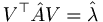$V^{\top}\hat{A}V=\hat{\lambda}$. It can then be converted back by inverting this equation: 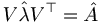$V\hat{\lambda}V^{\top}=\hat{A}$. This has two main advantages. The first is that any operator can be turned into a sum of its eigenfunctions and eigenvalues: $\hat{A}=\sum\vec{v}\lambda\vec{v^{\top}}$. The second is that many functions that would normally be difficult to compute on $\hat{A}$, like the exponential or trig functions, can be applied to $\hat{\lambda}$, which is then converted back using the original eigenvectors.

Note that this "diagonalization" actually amounts to changing into a new basis formed by the eigenvectors. This whole process is effectively like a very complex rotation of vectors.

Bra-ket Notation

Some people will understand the concepts involved much better now, and some won't. Since the point of this article is to reach the people who don't understand all of what's going on, here is a guide to manipulating bras and kets which should be much simpler to understand.