Badboys/shortlab
Building and testing of a NaI detector
Barrett Nibling, Adolfo Gomez, Micheal Bouchey
February 20, 2008
Contents |
Abstract
The purpose of this lab was to familiarize ourselves with scintillation detectors. This goal of understanding was accomplished by constructing, troubleshooting, and testing the important parameters of an NaI(Ti) detector. NaI detectors are used to detect gamma wave radiation given off from radio active gamma decay. The detector is built using an NaI crystal, from which it gets its name. Attached to the NaI crystal is a photomultiplier tube, which should be completely shielded from light in order to prevent ambient light from saturating the detector. In order to test for the proper function of the NaI detector, we performed experiments with two sources, a Cesium-137 source and a Cobalt-60 source. We used the Cesium source to find whether the proportionality for intensity with distance obeys  . The same source was also used to test the peak shaping and resolution of the NaI detector. The Cobalt-60 was used for the energy calibration of the detector and to ensure the detector was functioning properly using a Multichannel analyzer. The data we collected demonstrates that all of these aspects of functionality of the NaI detector work reasonably well. The data we collected also demonstrates the inverse-square law reasonably well. Our resolution was also well under 10% for all values.
List of Figures
- Figure 1 - Experimental Setup
- Figure 2 - Wiring Diagram
Introduction
The purpose of this lab is to construct and troubleshoot an NaI(Ti) scintillator detector. This detector is used to measure gamma wave radiation emitted from radioactive gamma decay. The construction of the detector is done by attaching an NaI crystal, from which the name of the detector is derived to a photomultiplier tube and then sealed completely to prevent light from entering and saturating the detector. Using a Cs-137 source we experimentally derived the resolution and the peak shaping of the detector as well as testing for the proportionality of the detector. Finally a Co-60 source was used for the energy calibration of the detector.
Theory
In order to detect a Gamma emission, a NaI(Ti) detector uses the photoelectric effect to measure the energy level of the incoming rays. This light created is then converted into photoelectrons inside the PM, accelerated with an electric field, and cascaded along many electrodes. This will create electrical pulses, which will get amplified, and can than be interpreted through a MCA. These pulses will be different varying the source used, the rate of which the source's gamma rays hits the detector. The higher the rate, the higher the intensity, therefore, the photo peak will be in turn higher. This is easily explained through the photoelectric effect that occurs in the detector. The higher the energy of the incoming particles, the more light that is admitted from the photoelectric effect, along with the constant amplification that occurs. Using this knowledge, we will be about to switch sources, keeping amplification the same, and compare the result. Then referencing previous results, we should then be able to calibrate our detector.
Procedure
Mounting the Crystal
1.Using electrical tape, tape the Photomultiplier (PM) to its base.
2.Carefully clean the PM with alcohol and then crystal with just the chemical wipes. Grease the contacts between the PM and crystal (just enough to cover).
3.Tape the whole thing with electrical tape to keep any light from possibly entering the PM. As well as apply an aluminum shield around the contraption.
4.Place in metal tubing, and mount on track (Fig.1).

Fig. 1 - Experimental Setup
Experimental Procedure
5.Connect the following- the high voltage input of the PM base to the HV output of the HV power supply and the anode output of the PM base to the oscilloscope. Turn on the HV power supply and turn up the voltage in steps of 100 V to a maximum of 1000V. Sketch the signal on the oscilloscope and give the rise time, fall time, and noise.
6.Disconnect the anode signal from the oscilloscope and connect it to the spectroscopy amplifier input. Power up the NIM bin and connect the oscilloscope to the amplifier output and sketch the signal.
7.Connect the unipolar output to the ADC/MCA input and start a measurement. The final setup should be wired according to Fig. 2. Adjust the gain so that the photo peak will be clear. Sketch the spectrum. With a likable gain, check the signal with the oscilloscope once again and record the voltage of the photo peak.

Fig. 2 - Wiring Diagram
8.Determine the average net count rate at various distances, checking to see if the 1/r2 law applies.
9.Calculate the resolution of the detector-system. By dividing the average full width half maximum (FWHM) of the photo peak by the average peak position. Record values for the resolution at several shaping times.
10.Select a gain that will fit the expected values from the 60-Co source on the spectrum. Print the 137-Cs spectrum at this gain.
11.Change the source to 60-Co. Measure the photo peak and print the spectrum.
12.Using the known peaks from both sources, compute the energy calibration for these detectors and electronic settings.
Results
The following tables contain the data recorded for the 137-Cs source. Three trials were taken for each distance with the averaged results listed.
Results 1
Table One:
| Trial | Peak | FWHM | Net CPS | Net Area | Area ± | Time (s) | Error (I) |
|---|---|---|---|---|---|---|---|
| 1 | 1594.95 | 108.54 | 56.45 | 16490 | 643 | 103 | 6.24 |
| 2 | 1595.27 | 108.53 | 56.29 | 16889 | 654 | 116 | 5.63 |
| 3 | 1596.92 | 123.63 | 56.74 | 17629 | 661 | 128 | 5.16 |
| Average | 1595.71 | 113.57 | 56.49 | 17003 | 653 | 116 | 5.68 |
Table Two:
| Trial | Peak | FWHM | Net CPS | Net Area | Area ± | Time (s) | Error (I) |
|---|---|---|---|---|---|---|---|
| 1 | 1050.45 | 77.08 | 52.75 | 5612 | 261 | 107 | 2.44 |
| 2 | 1059.67 | 72.71 | 53.00 | 3177 | 211 | 60 | 3.51 |
| 3 | 1061.71 | 79.71 | 51.86 | 6792 | 310 | 130 | 2.38 |
| Average | 1057.28 | 76.50 | 52.54 | 5194 | 261 | 99 | 2.77 |
Table Four:
| Trial | Peak | FWHM | Net CPS | Net Area | Area ± | Time (s) | Error (I) |
|---|---|---|---|---|---|---|---|
| 1 | 1055.63 | 2.70 | 8.21 | 1007 | 226 | 122 | 1.85 |
| 2 | 1055.52 | 5.77 | 7.37 | 1055 | 250 | 143 | 1.75 |
| 3 | 1055.57 | 2.69 | 7.40 | 1121 | 255 | 151 | 1.69 |
| Average | 1055.57 | 3.72 | 7.66 | 1061 | 244 | 139 | 1.78 |
Results 2
Error Analysis
For the error analysis, there are two variable associated with an error, θd and θi.
The partial errors for each of the variable are calculated from the formulas
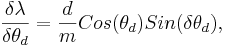
and,
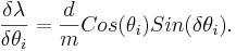
Then the total error is the sum of the two partial derivatives added in quadrature,
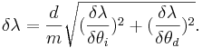
The values for δθd and δθi used are half the value of the smallest unit of measure on the device, .05 degrees.
Conclusion
The purpose of this lab was to familiarize ourselves with scintillation detectors. This goal of understanding was accomplished by constructing, troubleshooting, and testing the important parameters of an NaI(Ti) detector. NaI detectors are used to detect gamma wave radiation given off from radio active gamma decay. The detector is built using an NaI crystal, from which it gets its name. Attached to the NaI crystal is a photomultiplier tube, which should be completely shielded from light in order to prevent ambient light from saturating the detector. In order to test for the proper function of the NaI detector, we performed experiments with two sources, a Cesium-137 source and a Cobalt-60 source.
We were able to observe that the count rate was proportional to the distance by the proportion of with low error well under 15%. We were also able to observe a resolution well under the required 10%, our average resolutions ranged from 6.91% to 8.43%. Our calibration data from the Co-60 source also turned out well, the calibration (energy/bin) being on the order of 1.1.
References
[1]
[2]