Badboys/compton
(→List of Figures) |
(→List of Figures) |
||
| Line 13: | Line 13: | ||
== List of Figures == | == List of Figures == | ||
| − | Fig. 1 - Experimental Setup | + | '''Fig. 1''' - Experimental Setup |
| − | Fig. 2 - Compton Interaction | + | '''Fig. 2''' - Compton Interaction |
| − | Fig. 3 - Feynman Diagram of Compton Scattering | + | '''Fig. 3''' - Feynman Diagram of Compton Scattering |
== Introduction == | == Introduction == | ||
Revision as of 05:25, 3 April 2008
Compton Effect
Barrett Nibling, Adolfo Gomez, Micheal Bouchey
April 2, 2008
Contents |
Abstract
The Compton effect is the decrease in energy of a gamma ray photon when it interacts with matter. In this experiment 137-Cs gamma rays, emitted at approximately 0.662 MeV, strike an aluminum rod to produce measurable differences in the recorded energy of scattered gamma rays. The set of procedures is designed to investigate the experimental techniques used to measure the effects of Compton scattering. Using a NaI(T1), photomultiplier tube, ADC/MCA system, and a goniometer - data was collected at various incident angles. Calculated results agree with measured results within an accepted error value of XXXORALCOMPTONXXX.
List of Figures
Fig. 1 - Experimental Setup
Fig. 2 - Compton Interaction
Fig. 3 - Feynman Diagram of Compton Scattering
Introduction
intro here
Theory
Theory here
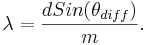
Example Math:
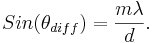
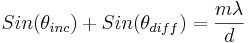 ,
,
Procedure
procedure here
Example Image:

Results
Data here
Results 1
Example Table
The First Order Spectrum:
| Color | θdiff (degrees) | λ (nm) | Error (nm) | Published λ (nm) | |
|---|---|---|---|---|---|
| Purple | 15.6 | 448.0 |  2.0 2.0
|
447.148 | |
| Teal | 16.4 | 470.3 | 2.0
|
471.314 | |
| Green | 17.2 | 492.6 | 2.0
|
492.193 | |
| Green | 17.5 | 500.9 | 2.0
|
501.567 | |
| Yellow//Orange | 20.7 | 588.8 | 2.0
|
587.562 | |
| Red | 23.6 | 666.9 | 2.0
|
667.815 | |
| Dim Red | 25.1 | 706.7 | 1.9
|
??? |
Results 2
Error Analysis
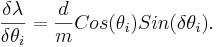
For the error analysis, there are two variable associated with an error, θd and θi.
The partial errors for each of the variable are calculated from the formulas
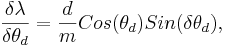
and,
Then the total error is the sum of the two partial derivatives added in quadrature,
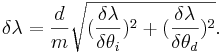
The values for δθd and δθi used are half the value of the smallest unit of measure on the device, .05 degrees.
Conclusion
conclusion here
References
[1]
[2]