Badboys/compton

Compton Effect

Barrett Nibling, Adolfo Gomez, Micheal Bouchey

April 2, 2008

---

Abstract

The Compton effect is the decrease in energy of a gamma ray photon when it interacts with matter. In this experiment 137-Cs gamma rays, emitted at approximately 0.662 MeV, strike an aluminum rod to produce measurable differences in the recorded energy of scattered gamma rays. The set of procedures is designed to investigate the experimental techniques used to measure the effects of Compton scattering. Using a NaI(T1), photomultiplier tube, ADC/MCA system, and a goniometer - data was collected at various incident angles. Calculated results agree with measured results within an accepted error value of XXXORALCOMPTONXXX.

List of Figures

Fig. 1 - Experimental Setup

Fig. 2 - Compton Interaction

Fig. 3 - Wiring Diagram

Introduction

Compton scattering, discovered in 1923 by Arthur Holly Compton, has both theoretical import and practical application. Compton's experimental results first proved that electromagnetics could not be explained solely as a wave phenomenon. When electromagnetic radiation interacts with matter, in particular electrons, the result is an increase in both the electron energy and in the wavelength of the emitted photon. An increase in wavelength is associated with a decrease in energy, suggesting that the photon lost some of its energy to the electron upon interacting. Furthermore, the effects of Compton scattering obey conservation of momentum. These results forced physicists to accept the duality of the nature of light.

The Compton effect has since been harnessed to provide useful technologies in the fields of astronomy, medicine, and of course physics. The reverse interaction, known as inverse Compton scattering, is observed in several cosmological phenomenon. Primarily, it is observed when photons travel through the cosmic microwave background. In medicine, X-ray scattering is the principle mechanism exploited in radiology. Gamma spectroscopy also relies on the principles of this effect.

This experiment is designed to study laboratory procedures used to acquire data. Measured results will be compared to calculated figures to determine systematic error. There are multiple sources for error in this experiment, most of which can be attributed to devices in the experimental setup.

Theory

Theory here

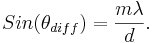
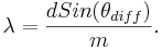
Example Math:

$Sin(\theta_{inc})+ Sin(\theta_{diff})=\frac{m \lambda}{d}$,

$Sin(\theta_{diff})=\frac{m \lambda}{d}.$

$\lambda = \frac{d Sin(\theta_{diff})}{m}.$

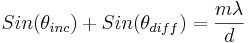Procedure

procedure here

Example Image:

Schematic of Spectroscopy Apparatus

Results

Data here

Results 1

Example Table

The First Order Spectrum:

Helium, d=1/600mm, m=1

Color	θdiff (degrees)	λ (nm)	Error (nm)	Published λ (nm)
Purple	15.6	448.0	$\pm$2.0	447.148
Teal	16.4	470.3	$\pm$2.0	471.314
Green	17.2	492.6	$\pm$2.0	492.193
Green	17.5	500.9	$\pm$2.0	501.567
Yellow//Orange	20.7	588.8	$\pm$2.0	587.562
Red	23.6	666.9	$\pm$2.0	667.815
Dim Red	25.1	706.7	$\pm$1.9	???

Error Analysis

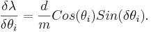
For the error analysis, there are two variable associated with an error, θ_d and θ_i.

The partial errors for each of the variable are calculated from the formulas

$\frac{\delta \lambda}{\delta \theta_{d}}=\frac{d}{m}Cos(\theta_{d})Sin({\delta \theta_{d}}),$

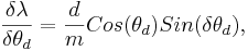
and,

$\frac{\delta \lambda}{\delta \theta_{i}}=\frac{d}{m}Cos(\theta_{i}) Sin({\delta \theta_{i}}).$

Then the total error is the sum of the two partial derivatives added in quadrature,

$\delta \lambda=\frac{d}{m} \sqrt{(\frac{\delta \lambda}{\delta \theta_{i}})^{2}+(\frac{\delta \lambda}{\delta \theta_{d}})^{2}}.$

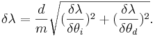
The values for δθ_d and δθ_i used are half the value of the smallest unit of measure on the device, .05 degrees.

Conclusion

Using a rudimentary goniometer and antiquated scientific apparatus, experimental procedure was deigned to minimize error. As a result, the measured results agreed with calculated values within a margin of XXX2GIRLS1CUPXXX. In a more advanced experiment, increasing the accuracy with which the angle is measured would most significantly affect data. However, other sources of error could also be improved with more sophisticated electronics. This lab provides an effective insight to the import of experimental procedure and equipment.

References

[1]

[2]