Badboys/alphagamma

Alpha and Gamma Cawinkadink

Barrett Nibling, Adolfo Gomez, Micheal Bouchey

March 20, 2008

---

Abstract

abstract here

List of Figures

• figure 1

• figure 2

• figures 3

Introduction

intro here

Theory

Theory here

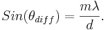
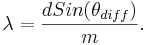
Example Math:

$Sin(\theta_{inc})+ Sin(\theta_{diff})=\frac{m \lambda}{d}$,

$Sin(\theta_{diff})=\frac{m \lambda}{d}.$

$\lambda = \frac{d Sin(\theta_{diff})}{m}.$

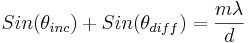Procedure

1.\tBuild a vacuum system (using one aluminum cube) with a port for a semiconductor detector on one end and a port for a radioactive alpha source on the opposite end. Connect the cube the existing pumping setup.\n 2.The semiconductor detector is mounted on a special extension to bring it near the alpha source position on the other side in vacuum. 3.The 241-Am source is mounted with a special flange that has an outside port fir the low energy gamma detector. This detector has a relatively small crystal optimized for the app. 60 keV gamma rays encountered in this experiment. 4.Close and evacuate the system with the roughing pump (to about 7 mTorr). 5.Connect: preamplifier to semiconductor detector feed-through: preamp output T to oscilloscope; preamp power to the outlet at the back of the amplifier. Power up the NIM bin. Connect the high voltage cable to the NIM HV power supply. Monitor the electric noise level of the amplifier signal on the oscilloscope while slowly turning the voltage up to +40 V. Describe what you see. Describe and sketch the signal seen on the oscilloscope: risetime, falltime, noise. 6.In order to shape and amplify the signals further for data acquisition, connect the preamp output to the amplifier input. Select the correct polarity on the polarity switch. Connect the unipolar output to the oscilloscope. Describe and sketch the signal seen on the oscilloscope: risetime, falltime, noise. What changes with using the gain switch and the shaping-time switch? Adjust the gain to a signal of 6 V for the highest alpha energies. 7.Startup the data acquisition program for the PC. Connect the unipolar output of the amplifier to the ADC/MCA input. Start the data acquisition and take a spectrum of the 241-Am source signal. Save for future printout on floppy disk. 8.Mount the scintillation detector in the slot prepared for it. This detector has a built in photomultiplier base (base) connected to the photomultiplier (PM). 9.Connect the signal output cable of the PM base to the oscilloscope. Check for a signal. 10.Connect the high voltage (HV) input cable of the PM base to the HV output of the HV power supply. 11.Turn on the HV power supply. Try to see the signals by adjusting the voltage in +100 V increments. Do not exceed +1200 V. 12.Take notes of the results and sketch the signals visible on the oscilloscope at +1000 V. Describe and sketch the signal seen on the oscilloscope: risetime, falltime, noise. 13.Connect the signal to the spectroscopy amplifier input. Check input signal polarity. 14.Connect the oscilloscope to the amplifier output (unipolar). Sketch the signal. 15.Connect the unipolar output with the ADC/MCA input and start a measurement. Adjust the amplification so that you can clearly see the signal peak in the spectrum. Save to disk for future printout. Sketch the spectrum. Check the signal again on the oscilloscope. Record the voltage of the photo peak. 16.Connect the output of the semiconductor amplifier to the input of the TSCA. Check with the oscilloscope if negative output pulses are produced. 17.Connect the bipolar output of the scintillator amplifier to the input of the other TSCA. Check again with the oscilloscope if negative output pulses are produced. 18.Connect additionally the unipolar output of the amplifier to the oscilloscope and trigger with the TSCA output. Try to set the TSCA window on the dominant approximately 60 keV signal. Introduce a delay into the TSCA and record the effect. 19.Connect the semiconductor line TSCA output to the start input of the TAC. Check with the oscilloscope if a valid start signal is registered. 20.Connect the scintillator line TSCA output to the stop input of the TAC. Select a 2 μs delay time at the TSCA. Select a full-scale time range of 10 μs at the TAC. 21.Monitor the TAC output on the oscilloscope. Describe and sketch it. 22.Connect the TAC output of the ADC/MCA and take a spectrum for approximately 1 hour. 23.Save the spectrum onto floppy disk for future printout and analysis. 24.In order to calibrate the time spectrum, introduce and additional delay in the form of a long cable or a NIM module in the scintillator line between TSAC ad TAC. 25.Take another spectrum for about one hour.

Results

Data here

Results 1

Example Table

The First Order Spectrum:

Helium, d=1/600mm, m=1

Color	θdiff (degrees)	λ (nm)	Error (nm)	Published λ (nm)
Purple	15.6	448.0	$\pm$2.0	447.148
Teal	16.4	470.3	$\pm$2.0	471.314
Green	17.2	492.6	$\pm$2.0	492.193
Green	17.5	500.9	$\pm$2.0	501.567
Yellow//Orange	20.7	588.8	$\pm$2.0	587.562
Red	23.6	666.9	$\pm$2.0	667.815
Dim Red	25.1	706.7	$\pm$1.9	???

Error Analysis

For the error analysis, there are two variable associated with an error, θ_d and θ_i.

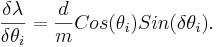
The partial errors for each of the variable are calculated from the formulas

$\frac{\delta \lambda}{\delta \theta_{d}}=\frac{d}{m}Cos(\theta_{d})Sin({\delta \theta_{d}}),$

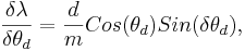
and,

$\frac{\delta \lambda}{\delta \theta_{i}}=\frac{d}{m}Cos(\theta_{i}) Sin({\delta \theta_{i}}).$

Then the total error is the sum of the two partial derivatives added in quadrature,

$\delta \lambda=\frac{d}{m} \sqrt{(\frac{\delta \lambda}{\delta \theta_{i}})^{2}+(\frac{\delta \lambda}{\delta \theta_{d}})^{2}}.$

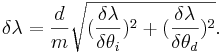
The values for δθ_d and δθ_i used are half the value of the smallest unit of measure on the device, .05 degrees.

Conclusion

conclusion here

References

[1]

[2]