The quantized harmonic oscillator

Course Wikis

>

Physics Course Wikis

>

Modern 2

Here the first key idea. Suppose you have a lattice of masses connected by springs.

or Buckyball

The natural coordinates are the displacements of the masses from their respective equilibria: $x_1, x_2 \$. In these coordinates the differential equations describing the motion of the system are coupled. However, if we solve these equations (which we will do in class), we find two solutions, one for which the motion is symmetric (both masses move in unison) and one antisymmetric (two masses move out of phase). These solutions have well defined frequencies ω₁,ω₂, hence in QM they would be eigenstates of the Hamiltonian. Since there are only two masses, the two solutions can be written as length-2 vectors (1,1),(1, − 1). It is a fundamental result that if we use the matrix that you get from putting these two eigenstates together, it defines a transformation into a new coordinate system in which the motion of the masses is completely decoupled.

The two motions of constant frequency are called normal modes in classical physics and energy eigenstates in quantum mechanics. For most problems of physical interest it is possible to construct normal modes that are mutually orthogonal. This means that the if you initialize the system in one of its modes, it will stay there forever since there is no coupling amongst the modes.

Thinking about normal modes can always be reduced to thinking about simple harmonic oscillators.

Here is an advanced example from Marlan O. Scully and M. Suhail Zubair Quantum Optics

page 1 page 2 page 3

compare Equation 1.1.9 of Scully and Zubari with equation 4.8 in your book.

1.1.9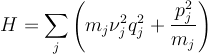 $H = \sum _ j \left( m_j \nu_j ^2 q_j ^2 + \frac{p_j ^2}{m_j} \right)$

4.8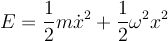 $E = \frac{1}{2} m \dot{x}^2 + \frac{1}{2} \omega^2 x^2$

But the argument above shows that if we have N coupled oscillators, we can always change coordinates and uncouple them. The new coordinates are given by the normal modes of the system. So, 1.1.9 also applies to a solid lattice!

Download Diagonalizing two coupled masses

here is another key idea: modes are fundamental in linear systems

first picture shows the ultrasonic impulse reponse of a rock excited and measured with lasers.

Next you see at the bottom of the figure, the Fourier transform of the impulse response. Above that you see a frequency-domain measurement (i.e., spectroscopy).

The top and bottom are similar. In fact they show the same modes, but in the top the frequencies are systematically lowered due to the mechanical loading of transducers. The bottom, being a purely optical measurement does not have this problem.

after a great earthquake the Earth rings like a bell

and how about the Sun!

At this point, I will switch to the board and review the classical problem of N coupled harmonic oscillators. We will pick up with the quantum problem on the Monday after Spring break.

Here are the pdf notes I will be following:

Download PDF Notes