Modern 2:Overview of Chapter 3
(→Physical Quantities and Observables) |
(→key ideas on measurement) |
||
| Line 7: | Line 7: | ||
* On the other hand, if we perform an experiment, the system will be in some state. How do we obtain as much information about this state. | * On the other hand, if we perform an experiment, the system will be in some state. How do we obtain as much information about this state. | ||
* Finally, we may wish to perform an experiment on a system in a ''given state''; i.e., one that is prepared experimentally to have well-defined properties. | * Finally, we may wish to perform an experiment on a system in a ''given state''; i.e., one that is prepared experimentally to have well-defined properties. | ||
| + | |||
| + | |||
| + | ==outcomes and probabilities== | ||
| + | |||
| + | ==repeatability of a measurement== | ||
| + | |||
| + | If we measure a quantity ''A'' at some time ''t'' and find that the result is ''a'', then we assume that if we measure this quantity again at a time just after ''t'', we must get the same result. That means that in the second case the probability of getting ''a'' in the measurement was 1. In general that cannot be the case for the first measurment. The logical implication of this is that the measurement itself has transformed the system into a new state: it has been transformed into a state on which measurment of ''A'' gives ''a'' with certainty. Page 41 of the book. | ||
==reminder from chapter 2== | ==reminder from chapter 2== | ||
Revision as of 01:16, 24 February 2006
Contents |
Overview of Chapter 3
2/24/06
key ideas on measurement
- The state of a system is system is described by a wavefunction. ψ(r,t). The wavefunction evolves deterministically according to the Schrodinger equation. However, we give a probabilistic interpretation to the wave function that allows us to predict the measurement of a given physical quantity.
- On the other hand, if we perform an experiment, the system will be in some state. How do we obtain as much information about this state.
- Finally, we may wish to perform an experiment on a system in a given state; i.e., one that is prepared experimentally to have well-defined properties.
outcomes and probabilities
repeatability of a measurement
If we measure a quantity A at some time t and find that the result is a, then we assume that if we measure this quantity again at a time just after t, we must get the same result. That means that in the second case the probability of getting a in the measurement was 1. In general that cannot be the case for the first measurment. The logical implication of this is that the measurement itself has transformed the system into a new state: it has been transformed into a state on which measurment of A gives a with certainty. Page 41 of the book.
reminder from chapter 2
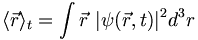
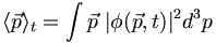
But we can also compute the expectation of p in position space. This is essential if we want to be able to treat variables such as angular momentum, which involve both position and momentum: 
Here is a fundamental result which you should prove:
(3.3) 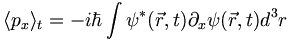
 means partial with respect to x. And henceforth, equation numbers such as 3.3 above will refer to the equation number in the text.
The general vector form of 3.3 is the following:
(3.4) 
The reason I put brackets around the  is that we can consider this operator as
being the position space representation of
is that we can consider this operator as
being the position space representation of  .
.
(3.9)
Physical Quantities and Observables
vectors and operators
We're going to build up to the definition of an operator, but
let's start with the idea of physical vectors. These are objects that have a direction and length (or magnitude). The force on an object for example. In a particular coordinate system we can represent this vector as a 3-tuple. E.g., 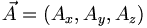 . So the 3-tuple is the representation of the vector in a particular coordinate system. In other coordinates there will be other tuples, but the vector itself has an existance independent of the coordinates used.
So the way to think of a vector equation such as  is that the object A is mapping one vector into another. If the vectors have the same length, then A can be represented by a square matrix. In the same way, we can think of functions as vectors too. Just as we add vectors component-wise:
![[\vec{x} + \vec{y}] _ i = x_i + y_i](/csm/wiki/images/math/6/b/5/6b5b0ae8acc4837872df10a4359b1553.png)
we add functions point-wise. If f and g are functions of one variable, then
[f + g](x) = f(x) + g(x)
The main difference between these two equations is that the functions, in effect, have an infinite number of components, one for each value of the real variable x!
Now we can consider operators acting not on finite