Modern 2:Overview of Chapter 3
(Difference between revisions)
(→Overview of Chapter 3) |
|||
| Line 15: | Line 15: | ||
Here is a fundamental result '''which you should prove''': | Here is a fundamental result '''which you should prove''': | ||
| − | <math> \langle p _x \rangle _ t = -i \hbar \int \psi^*(\vec{r},t) \partial _x \psi(\vec{r},t) d^3 r </math> | + | |
| + | '''(3.3)''' <math> \langle p _x \rangle _ t = -i \hbar \int \psi^*(\vec{r},t) \partial _x \psi(\vec{r},t) d^3 r </math> | ||
<math> \partial _x </math> means partial with respect to <math>x</math>. And henceforth, equation numbers such as 3.4 above will refer to the equation number in the text. | <math> \partial _x </math> means partial with respect to <math>x</math>. And henceforth, equation numbers such as 3.4 above will refer to the equation number in the text. | ||
| Line 22: | Line 23: | ||
The general vector form of 3.3 is the following: | The general vector form of 3.3 is the following: | ||
| − | <math> \langle \vec{p} \rangle _ t = -i \hbar \int \psi^*(\vec{r},t) \nabla \psi(\vec{r},t) d^3 r = \int \psi^*(\vec{r},t) \left( \hbar/i \nabla \right) \psi(\vec{r},t) d^3 r </math> | + | '''(3.4)''' <math> \langle \vec{p} \rangle _ t = -i \hbar \int \psi^*(\vec{r},t) \nabla \psi(\vec{r},t) d^3 r = \int \psi^*(\vec{r},t) \left( \hbar/i \nabla \right) \psi(\vec{r},t) d^3 r </math> |
The reason I put brackets around the <math> \hbar /i \nabla</math> is that we can consider this operator as | The reason I put brackets around the <math> \hbar /i \nabla</math> is that we can consider this operator as | ||
being the position space representation of <math>\vec{p}</math>. | being the position space representation of <math>\vec{p}</math>. | ||
Revision as of 00:41, 24 February 2006
Overview of Chapter 3
2/24/06
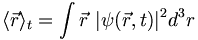
- The state of a system is system is described by a wavefunction. ψ(r,t). The wavefunction evolves deterministically according to the Schrodinger equation. However, we give a probabilistic interpretation to the wave function that allows us to predict the measurement of a given physical quantity.
- On the other hand, if we perform an experiment, the system will be in some state. How do we obtain as much information about this state.
- Finally, we may wish to perform an experiment on a system in a given state; i.e., one that is prepared experimentally to have well-defined properties.
Reminder
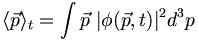
But we can also compute the expectation of p in position space. This is essential if we want to be able to treat variables such as angular momentum, which involve both position and momentum: 
Here is a fundamental result which you should prove:
(3.3) 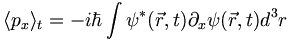
 means partial with respect to x. And henceforth, equation numbers such as 3.4 above will refer to the equation number in the text.
The general vector form of 3.3 is the following:
(3.4) 
The reason I put brackets around the  is that we can consider this operator as
being the position space representation of
is that we can consider this operator as
being the position space representation of  .
.