Classical vs quantum harmonic oscillator. Correspondance principle
(→Now let's look at some of the quantum harmonic oscillator states) |
m (Reverted edit of Dmurrell, changed back to last version by Rinman) |
||
| (24 intermediate revisions by 4 users not shown) | |||
| Line 5: | Line 5: | ||
===some key ideas on the harmonic oscillator=== | ===some key ideas on the harmonic oscillator=== | ||
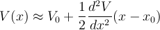
| − | * <math> \omega | + | * <math> \omega </math> is the natural frequency of the oscillator. This |
| − | is a property of the potential. Remember, for small displacements from | + | is a property of the '''potential'''. Remember, for small displacements from |
equilibrium: <math> x_0</math>. | equilibrium: <math> x_0</math>. | ||
| Line 18: | Line 18: | ||
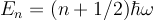
* in 1D the QHO has an infinite series of equally spaced energy levels: | * in 1D the QHO has an infinite series of equally spaced energy levels: | ||
| + | |||
<math> E_n = (n + 1/2) \hbar \omega </math> | <math> E_n = (n + 1/2) \hbar \omega </math> | ||
| − | * many of the calculations become simpler if we introduce dimensionless | + | * many of the calculations become simpler if we introduce dimensionless variables |
| − | variables | + | |
<math> \tilde{x} \equiv x \sqrt{m \omega/\hbar} </math> | <math> \tilde{x} \equiv x \sqrt{m \omega/\hbar} </math> | ||
| Line 32: | Line 32: | ||
This is a striking result since it says that for energy eigenstates, | This is a striking result since it says that for energy eigenstates, | ||
| − | nature will not allow us to | + | nature will not allow us to sacrifice knowledge of one variable, |
in order to gain knowledge of the other. | in order to gain knowledge of the other. | ||
| Line 51: | Line 51: | ||
In either case, the solution is: | In either case, the solution is: | ||
| − | <math> x(t) = A \cos(\omega _0 t + \Delta) </math> where <math>\Delta \ </math> is a phase factor. | + | <math> x(t) = A \cos(\omega _0 t + \Delta) \ </math> where <math>\Delta \ </math> is a phase factor. |
Now, from this solution it is not hard to show that the total energy is a constant: | Now, from this solution it is not hard to show that the total energy is a constant: | ||
| Line 57: | Line 57: | ||
<math> E = T + U = \frac{1}{2} m \dot{x} ^2 + \frac{1}{2} k x^2 </math> | <math> E = T + U = \frac{1}{2} m \dot{x} ^2 + \frac{1}{2} k x^2 </math> | ||
| − | Hence, <math> E = \frac{1}{2} m \omega_0 ^2 A ^2 \sin^2(\omega _0 t + \Delta) + \frac{1}{2} k | + | Hence, <math> E = \frac{1}{2} m \omega_0 ^2 A ^2 \sin^2(\omega _0 t + \Delta) + \frac{1}{2} k A ^2 \cos^2(\omega _0 t + \Delta) </math> |
| − | <math> = \frac{1}{2} k | + | <math> = \frac{1}{2} k A ^2 \sin^2(\omega _0 t + \Delta) + \frac{1}{2} k A ^2 \cos^2(\omega _0 t + \Delta) =\frac{1}{2} k A^2 </math> |
So, in the classical case (assuming no dissipation) we adjust the energy by adjusting how far we pull the mass from its equilibrium position. | So, in the classical case (assuming no dissipation) we adjust the energy by adjusting how far we pull the mass from its equilibrium position. | ||
| Line 73: | Line 73: | ||
{{mathematica|filename=HOstates.nb|title=several harmonic oscillator eigenstates}} | {{mathematica|filename=HOstates.nb|title=several harmonic oscillator eigenstates}} | ||
| − | Key idea: for small n, the mass is most likely to be near x=0. This is exactly the opposite of the classical case. However, for large n, the classical and quantum result are similar, with | + | Key idea: for small n, the mass is most likely to be near x=0. This is exactly the opposite of the classical case. |
| + | However, for large n, the classical and quantum result are similar, with a few exceptions. | ||
| + | |||
| + | * There are still nodes in | ||
| + | the probability due to the interference of the back and forth wave-like propagation of the particle. | ||
| + | |||
| + | * The limit of the classical motion is strictly <math>\pm A</math>. However, there is small but nonzero that | ||
| + | the quantum particle will be found outside this limit. This is another example of tunneling. | ||
| + | |||
| + | |||
| + | |||
| + | With <math>E_n = (n + 1/2) \hbar \omega</math>. To make the classical correspondance, we want: | ||
| + | |||
| + | <math> \frac{1}{2} K A ^2 = (n + 1/2) \hbar \omega</math>. Hence to get a classical oscillator with the same energy as the quantum oscillator we choose: | ||
| + | |||
| + | <math>A^2 = 2 (n + 1/2) \hbar \omega / (m \omega ^2) = 2 (n + 1/2) \hbar /(m \omega) </math>. But remember, <math>\hbar /(m \omega)</math> | ||
| + | is our basic unit of length (which we used to make the equations dimensionless). Hence in units of <math>\hbar /(m \omega)</math> we | ||
| + | want the amplitude of our classical spring to be <math> = \sqrt{2n}</math> (ignoring the small factor of <math>1/2</math>). | ||
| + | |||
| + | ===The Correspondance Principle=== | ||
| + | |||
| + | As n gets large, the quantum problem approaches the classical | ||
| + | |||
| + | Or, another way to think of this is: When is the discreteness of the energy levels, <math> \hbar \omega </math>, small enough to be ignored? | ||
| + | |||
| + | Other examples include Rydberg states for atoms. These are highly excited states with nearly spherical orbits. | ||
Latest revision as of 19:37, 8 February 2007
reminder: Jared Diamond talk next tuesday
some key ideas on the harmonic oscillator
- ω is the natural frequency of the oscillator. This
is a property of the potential. Remember, for small displacements from equilibrium: x0.
Hence the force associatd with the potential is:
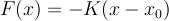
where 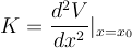
- in 1D the QHO has an infinite series of equally spaced energy levels:
- many of the calculations become simpler if we introduce dimensionless variables
In particular, you can show that:
Variance Variance
This is a striking result since it says that for energy eigenstates, nature will not allow us to sacrifice knowledge of one variable, in order to gain knowledge of the other.
Brief digression, the astounding cancelation properties of Hermite polynomials
| |
Classical versus Quantum harmonic oscillator
We've seen two ways to write the equations of motion for the classical SHO:
Newtonian:
Hamiltonian:
where 
In either case, the solution is:
 where
where  is a phase factor.
Now, from this solution it is not hard to show that the total energy is a constant:
Hence, 

So, in the classical case (assuming no dissipation) we adjust the energy by adjusting how far we pull the mass from its equilibrium position. Once we've done that, it oscillates in simple harmonic motion forever.
Where does the mass-on-a-spring spend most of its time
| |
Now let's look at some of the quantum harmonic oscillator states
| |
Key idea: for small n, the mass is most likely to be near x=0. This is exactly the opposite of the classical case.
However, for large n, the classical and quantum result are similar, with a few exceptions.
- There are still nodes in
the probability due to the interference of the back and forth wave-like propagation of the particle.
- The limit of the classical motion is strictly
 . However, there is small but nonzero that
the quantum particle will be found outside this limit. This is another example of tunneling.
With . To make the classical correspondance, we want:
 . Hence to get a classical oscillator with the same energy as the quantum oscillator we choose:
 . But remember,
  is our basic unit of length (which we used to make the equations dimensionless). Hence in units of we
want the amplitude of our classical spring to be
is our basic unit of length (which we used to make the equations dimensionless). Hence in units of we
want the amplitude of our classical spring to be  (ignoring the small factor of 1 / 2).
The Correspondance Principle
As n gets large, the quantum problem approaches the classical
Or, another way to think of this is: When is the discreteness of the energy levels,  , small enough to be ignored?
Other examples include Rydberg states for atoms. These are highly excited states with nearly spherical orbits.