Badboys/attenuation

(Difference between revisions)

Jump to: navigation, search

Revision as of 07:55, 7 February 2008

Gamma Ray Attenuation

Barrett Nibling, Adolfo Gomez, Micheal Bouchey

February 6, 2008

Abstract

This experiment uses an NaI(T1) to determine mass attenuation coefficients for lead and aluminum, for 662 keV gamma rays, which are then compared to published values. The error present in the measurements is less than XX%, and published values agree with experimental results within that error.

List of Figures

Fig. 1 - Experimental Setup

Introduction

intro here

Theory

Gamma attenuation occurs in a variety of ways. When Gamma rays travel through a barrier, attenuation is caused by photoelectric or Compton interactions with the material. In this lab these interactions are between the gamma rays and the Aluminum or Lead barriers placed in between the Cesium source and the gamma ray spectrometer. Lambert’s law gives the intensity of the radiation after it has passed through the barrier as[1]:

$I = I 0 e - μ x$ ,

Where:

I = intensity of the radiation after it has passed through the barrier

$I 0$ = initial intensity of the radiation before it has passed through the barrier

µ = total mass attenuation coefficient with units of cm^2/g

x = density thickness with units of g/cm^2

This density thickness is the product of the density of the material and the thickness of the barrier.

In this particular experiment we can measure I, $I 0$ , and x and must use equation (1) to calculate the attenuation coefficient.

The half-value layer (HVL) is defined as the density thickness of the absorbing material that will reduce the original intensity by a factor of two. Once µ is calculated HVL can be calculated with[2]:

$0.5 = - μ x$

Where:

0.5 = the ratio of I/ $I 0$ . It must be one-half to represent the reduction of the intensity by a factor of two

µ = total mass attenuation coefficient calculated from equation (1)

x = HVL

The gamma ray spectrometer works by photon emissions from excited electrons. The gamma rays that make it to the spectrometer are absorbed by electrons, moving these electrons in to excited states. As these electrons leave their excited state they emit photons which are measured by the spectrometer. The resulting readings look like a downward spike, when using the anode on the spectrometer, with a very steep initial slope because the beginning of the measurement has a very small time difference between no photon emissions and when the electrons first begin to emit photons, and a quadratic rising decay back to zero because electrons can only emit photons once if they are only excited once and so as more electrons emit photons, there are less electrons remaining to emit more photons. We observed this process at step 5 in our provided lab procedure.

We see a similar signal when using the dynode on the spectrometer but because the dynode is positively charged the spike is in the positive direction instead of the negative direction. The dynode itself is positive because it is used to amplify the cathode signal [3].

Procedure

1. Mount the NaI(TI) detector and the 137-Cs source with a distance of approximately 30 cm. The center of the source should be on the same height as the center of the detector crystal. Connect the photomultiplier base (base) to the photomultiplier (PM) connector.

2. Connect the high voltage (HV) imput of te PM base to the HV output of the HV power supply.

3. Connect the anode output of the PM base to the oscilloscope. At this point we observed a flat line signal.

4. Turn on the HV power supply. The screw or switch on the back side should be on positive. Turn up the voltage in increments of 100V to a maximum of 1000V and observe the signals on the oscilloscope. We did not notice anything observable until 1000V

5. Take specific notes of results for the signals on the oscilloscope at 1000V. We observed a spike in the negative direction. It is noteworthy to give a warning that the trigger level must be below zero or the oscilloscope will give a misleading reading.

6. Perform steps 3-5 using the dynode output of the PM instead of the anode output of the PM. We observed a spike in the positive direction this time. Again, noteworthy to give warning that this time the trigger level must be above zero or the oscilloscope will give a misleading reading.

7. Return to the anode signal and connect it to the spectroscopy amplifier input. Turn on the power of the NIM bin and check the input signal polarity.

8. Connect the oscilloscope to the amplifier output (unipolar). Making sure to again move the oscilloscope trigger level to below zero record the signal. We noted a similar signal to step 5.

9. Connect the unipolar output with the ADC input and start a measurement. Adjust the amplification so that you can clearly see the photopeak in the spectrum. Record the spectrum and the oscilloscope signal and record the voltage of the photopeak. We a spectrum with a large amount of noise in the low voltage range and our photopeak in the midvoltage range.

10. Determine the count rate (net) in the photopeak region at your given distance without the absorber foils. This is a zero measurement and will give I0.

11. Determine the count rate in the photopeak region with three absorber foils of aluminum and lead each. Take three measurements with each foil.

12. Calculate the attenuation coefficient using equation (1) and the half-value layer for lead and aluminum for 662 keV photons using equation (2).

Analysis

Data:

Lead Data:

Thickness Data- Lead
Sample #	Measurement 1 (mm)	Measurement 2 (mm)	Measurement 3 (mm)	Measurement 4 (mm)	Average (mm)	Error (mm)
Sample A	0.960	0.920	0.942	0.970	0.948	$\pm$ 0.005
Sample E	6.335	6.335	6.355	6.335	6.340	$\pm$ 0.005
Sample C	2.260	2.250	2.240	2.270	2.255	$\pm$ 0.005

Attenuation Data
Sample #	Average Thickness (mm)	Density ( $g / c m 3$ )	$I o$ (Count Rate)	$I 1$	$I 2$	$I 3$	Average $I$	$μ$ ( $c m 2 / g$ )	Error ( $c m 2 / g$ )	HVL
Sample A	0.948	11.434	90.59	75.54	75.92	73.03	74.83	0.01672	$\pm$ 0.005	41.45
Sample E	6.340	11.434	90.59	38.11	40.23	37.11	38.48	0.07487	$\pm$ 0.005	9.25
Sample C	2.255	11.434	90.59	62.25	64.50	63.75	63.50	0.03107	$\pm$ 0.005	22.30

Aluminum Data:

Thickness Data- Aluminum
Sample #	Measurement 1 (mm)	Measurement 2 (mm)	Measurement 3 (mm)	Measurement 4 (mm)	Average (mm)	Error (mm)
Size 24	5.115	5.020	5.010	5.030	5.044	$\pm$ 0.005
Size 8	0.421	0.420	0.422	0.411	0.419	$\pm$ 0.005

Attenuation Data
Sample #	Average Thickness (mm)	Density ( $g / c m 3$ )	$I o$ (Count Rate)	$I 1$	$I 2$	$I 3$	Average $I$	$μ$ ( $c m 2 / g$ )	Error ( $c m 2 / g$ )	HVL
Size 24	5.044	2.702	90.59	72.47	74.04	73.67	73.39	0.07791	$\pm$ 0.005	8.89
Size 8	5.044	2.702	90.59	84.45	84.81	84.04	84.43	0.02605	$\pm$ 0.005	26.60

Error Analysis

For the error analysis, there are For the error analysis, there are two variable associated with an error, $θ d$ and $θ i$ .

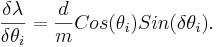
The partial errors for each of the variable are calculated from the formulas

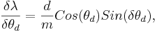
$\frac{\delta \lambda}{\delta \theta_{d}}=\frac{d}{m}Cos(\theta_{d})Sin({\delta \theta_{d}}),$

and,

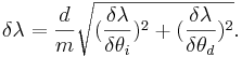
$\frac{\delta \lambda}{\delta \theta_{i}}=\frac{d}{m}Cos(\theta_{i}) Sin({\delta \theta_{i}}).$

Then the total error is the sum of the two partial derivatives added in quadrature,

$\delta \lambda=\frac{d}{m} \sqrt{(\frac{\delta \lambda}{\delta \theta_{i}})^{2}+(\frac{\delta \lambda}{\delta \theta_{d}})^{2}}.$

The values for $δθ d$ and $δθ i$ used are half the value of the smallest unit of measure on the device, .05 degrees.

Conclusion

conclusion here

References

[1]

[2]

@@ Line 13: / Line 13: @@
 == List of Figures ==
-*figure 1
-*figure 2
+[[Image:ExperimentalSetup1tn.jpg]]
+*Fig. 1 - Experimental Setup
-*figures 3[[Image:ExperimentalSetup1.jpg]]
 == Introduction ==

Badboys/attenuation

Revision as of 07:55, 7 February 2008

Contents

Abstract

List of Figures

Introduction

Theory

Procedure

Analysis

Data:

Lead Data:

Aluminum Data:

Error Analysis

Conclusion

References

Personal tools

Namespaces

Variants

Views

Actions

Search

Navigation

Toolbox