Badboys/alpha

(Difference between revisions)

Jump to: navigation, search

Revision as of 04:22, 21 February 2008

Alpha Particle Energy Loss

Barrett Nibling, Adolfo Gomez, Micheal Bouchey

February 20, 2008

Abstract

abstract here

List of Figures

figure 1

figure 2

figures 3

Introduction

intro here

Theory

Surface-Barrier Detectors

In this lab we are using an R-016-050-100 surface-barrier detector to measure the energy loss of alpha particles. The ORTEC model number mentioned above reflects three different parameters that are used to define a silicon surface-barrier detector. These parameters are resolution, active area, and depletion depth. In our model, the resolution is 16keV FWHM for 241-Am alphas, which comes from the 016. The active area is 50mm2, which comes from the 050. The depletion depth is 100µm, which comes from the 100.

Because the shape of the detector is a circular disk, the active area is the circular area of the face of the detector. At any distance from the source, a larger area means a larger angle and that means that more of the alpha particles emanating from the source will run in to the detector. This also implies that distance between the alpha source and the detector will affect the number of alpha particles that run in to the detector as well if the area is being held constant.

The depletion depth is the sensitive depth of the detector. The depth is important because it must be sufficient to completely stop all of the charged particles that are to be measured in the experiment. A 5.5MeV alpha particle is completely stopped with about 27µm of silicon. This means that, because natural alphas are usually less then 8MeV in energy, the 50µm detector used in this lab should stop all natural alphas.

Surface-barrier detectors are essentially 100% efficient for their active areas. This means that one can calculate the activity in alphas per second fairly easily

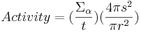
$Activity = (\frac{\Sigma_{\alpha}}{t}) (\frac{4 \pi s^2}{\pi r^2})$

Where

s = distance from source to detector

r = radius of the detector (cm)

t = time in seconds

Σα = counts in spectrum

1µCi = 3.7*104 disintegrations per second

Alpha Sources

In doing the experiment we see one peak for the Cm source. In reality a Cm source should show two peaks. This is because Cm is a very strong alpha source and so there is a thin metal foil over the Cm source for protection. The alpha particles loose energy in this foil which mean we cannot get an accurate base measurement from the Cm source. This is why there are two sources being used. The Po source is far less radioactive but is also unprotected and so it is used to gather our base reading.

The Cm source itself has a half-life of 18.1 years as opposed to the half-life of Po which is only 138 days. At 100% branching the Cm source has a Q-value of 5901.65 while the Po source has a Q-value of 5407.46. So the Cm source also has a much higher Q-value.

Procedure

1) Build a vacuum system with detector on one and a port for a radioactive alpha source on the other. Measure the distance between the alpha detector and the port for the radioactive source. The distance should be about 40cm, in our experiment the distance was 36.5 cm. Also connect a vacuum gauge, a roughing pump through a valve, and a needle valve for venting, to the vacuum system.

2) Test the vacuum system for leaks. The whole vacuum system should get below 10 torr. If this level is not reached, then there is likely a leak somewhere.

3) Set up the electronic equipment – connect:

a. Preamplifier to detector feed through

b. Preamp output E to oscilloscope

c. Preamp power to the outlet at the back of the amplifier

4) Once all the electronic equipment is set up, retrieve the source. The first source is Cm (Curium) which is shielded so it cannot be used for a base reading. The second source is Po (Polonium) which is not shielded and will be used for a base reading. Put the Cm in to the vacuum system for now.

5) Power up the NIM bin. Describe and sketch the signal seen on the oscilloscope including rise time, fall time, and noise.

6) Connect the preamp output to the amplifier input with the polarity set to positive. Connect the unipolar output to the oscilloscope and, again, describe and sketch the signal including rise time, fall time, and noise.

7) Connect the high voltage cable to the 0-500V output on the NIM HV power supply. Monitor the electronic noise level of the amplifier signal on the oscilloscope while slowly turning the voltage up to +40V.

8) Startup the MCDWIN data acquisition program on the PC. Connect the unipolar output of the amplifier to the ADC/MCA input and the oscilloscope to the bipolar output. Start the data acquisition and take a spectrum of the Cm source signal. Use print screen and save the image to a word document.

9) Determine the peak position and FWHM for the Cm source at the following pressures: 7 torr, 7.3 torr, 9.9 torr, 13 torr, 15 torr, 17.5 torr, and 20.1 torr. It is not required that these exact values be used, these are, however, the values we used in our experiment.

10) Turn off the gigh voltage and NIM bin power supply. Close the valve to the roughing pump and open the needle valve. Change to the Po source.

11) Evacuate the system. Turn HV and NIM bin back on. Monitor the oscilloscope and the ADC/MCA.

12) Calculate the anticipated count rate under the assumption of source a strength of 0.1 µCi.

13) Run this measurement for ½ hour at 6.9 torr and compare the result to the calculation from step 12.

Example Image:

Schematic of Spectroscopy Apparatus

Results

Data here

Results 1

Example Table

The First Order Spectrum:

Helium, d=1/600mm, m=1
Color	$θ d i f f$ (degrees)	$λ$ (nm)	Error (nm)	Published $λ$ (nm)
Purple	15.6	448.0	$\pm$ 2.0	447.148
Teal	16.4	470.3	$\pm$ 2.0	471.314
Green	17.2	492.6	$\pm$ 2.0	492.193
Green	17.5	500.9	$\pm$ 2.0	501.567
Yellow//Orange	20.7	588.8	$\pm$ 2.0	587.562
Red	23.6	666.9	$\pm$ 2.0	667.815
Dim Red	25.1	706.7	$\pm$ 1.9	???

Results 2

Error Analysis

For the error analysis, there are two variable associated with an error, $θ d$ and $θ i$ .

The partial errors for each of the variable are calculated from the formulas

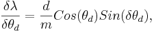
$\frac{\delta \lambda}{\delta \theta_{d}}=\frac{d}{m}Cos(\theta_{d})Sin({\delta \theta_{d}}),$

and,

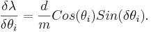
$\frac{\delta \lambda}{\delta \theta_{i}}=\frac{d}{m}Cos(\theta_{i}) Sin({\delta \theta_{i}}).$

Then the total error is the sum of the two partial derivatives added in quadrature,

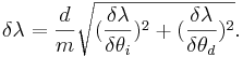
$\delta \lambda=\frac{d}{m} \sqrt{(\frac{\delta \lambda}{\delta \theta_{i}})^{2}+(\frac{\delta \lambda}{\delta \theta_{d}})^{2}}.$

The values for $δθ d$ and $δθ i$ used are half the value of the smallest unit of measure on the device, .05 degrees.

Conclusion

conclusion here

References

[1]

[2]

Badboys/alpha

Revision as of 04:22, 21 February 2008

Contents

Abstract

List of Figures

Introduction

Theory

Procedure

Results

Results 1

Results 2

Error Analysis

Conclusion

References

Personal tools

Namespaces

Variants

Views

Actions

Search

Navigation

Toolbox

@@ Line 66: / Line 66: @@
-procedure here
+)	Build a vacuum system with detector on one and a port for a radioactive alpha source on the other.  Measure the distance between the alpha detector and the port for the radioactive source.  The distance should be about 40cm, in our experiment the distance was 36.5 cm.  Also connect a vacuum gauge, a roughing pump through a valve, and a needle valve for venting, to the vacuum system.
+)	Test the vacuum system for leaks.  The whole vacuum system should get below 10 torr.  If this level is not reached, then there is likely a leak somewhere.
+)	Set up the electronic equipment – connect:
+a.	Preamplifier to detector feed through
+b.	Preamp output E to oscilloscope
+c.	Preamp power to the outlet at the back of the amplifier
+)	Once all the electronic equipment is set up, retrieve the source.  The first source is Cm (Curium) which is shielded so it cannot be used for a base reading.  The second source is Po (Polonium) which is not shielded and will be used for a base reading.  Put the Cm in to the vacuum system for now.
+)	Power up the NIM bin.  Describe and sketch the signal seen on the oscilloscope including rise time, fall time, and noise.
+)	Connect the preamp output to the amplifier input with the polarity set to positive.  Connect the unipolar output to the oscilloscope and, again, describe and sketch the signal including rise time, fall time, and noise.
+)	Connect the high voltage cable to the 0-500V output on the NIM HV power supply.  Monitor the electronic noise level of the amplifier signal on the oscilloscope while slowly turning the voltage up to +40V.
+)	Startup the MCDWIN data acquisition program on the PC.  Connect the unipolar output of the amplifier to the ADC/MCA input and the oscilloscope to the bipolar output.  Start the data acquisition and take a spectrum of the Cm source signal.  Use print screen and save the image to a word document.
+)	Determine the peak position and FWHM for the Cm source at the following pressures: 7 torr, 7.3 torr, 9.9 torr, 13 torr, 15 torr, 17.5 torr, and 20.1 torr.  It is not required that these exact values be used, these are, however, the values we used in our experiment.
+)	Turn off the gigh voltage and NIM bin power supply.  Close the valve to the roughing pump and open the needle valve.  Change to the Po source.
+)	Evacuate the system.  Turn HV and NIM bin back on.  Monitor the oscilloscope and the ADC/MCA.
+)	Calculate the anticipated count rate under the assumption of source a strength of 0.1 µCi.
+)	Run this measurement for ½ hour at 6.9 torr and compare the result to the calculation from step 12.